Project FOMC29493 services include NGS sequencing of the V1V3 region of the 16S rRNA gene amplicons from the samples. First and foremost, please
download this report, as well as the sequence raw data from the download links provided below.
These links will expire after 60 days. We cannot guarantee the availability of your data after 60 days.
Full Bioinformatics analysis service was requested. We provide many analyses, starting from the raw sequence quality and noise filtering, pair reads merging, as well as chimera filtering for the sequences, using the
DADA2 denosing algorithm and pipeline.
We also provide many downstream analyses such as taxonomy assignment, alpha and beta diversity analyses, and differential abundance analysis.
For taxonomy assignment, most informative would be the taxonomy barplots. We provide an interactive barplots to show the relative abundance of microbes at different taxonomy levels (from Phylum to species) that you can choose.
If you specify which groups of samples you want to compare for differential abundance, we provide both ANCOM and LEfSe differential abundance analysis.
The samples were processed and analyzed with the ZymoBIOMICS® Service: Targeted
Metagenomic Sequencing (Zymo Research, Irvine, CA).
DNA Extraction: If DNA extraction was performed, the following DNA
extraction kit was used according to the manufacturer’s instructions:
☑
ZymoBIOMICS®-96 MagBead DNA Kit (Zymo Research, Irvine, CA)
☐
N/A (DNA Extraction Not Performed)
Elution Volume: 50µL
Additional Notes: NA
Targeted Library Preparation: The DNA samples were prepared for targeted
sequencing with the Quick-16S™ NGS Library Prep Kit (Zymo Research, Irvine, CA).
These primers were custom designed by Zymo Research to provide the best coverage
of the 16S gene while maintaining high sensitivity. The primer sets used in this project
are marked below:
☐
Quick-16S™ Primer Set V1-V2 (Zymo Research, Irvine, CA)
☑
Quick-16S™ Primer Set V1-V3 (Zymo Research, Irvine, CA)
☐
Quick-16S™ Primer Set V3-V4 (Zymo Research, Irvine, CA)
☐
Quick-16S™ Primer Set V4 (Zymo Research, Irvine, CA)
☐
Quick-16S™ Primer Set V6-V8 (Zymo Research, Irvine, CA)
Additional Notes: NA
The sequencing library was prepared using an innovative library preparation process in
which PCR reactions were performed in real-time PCR machines to control cycles and
therefore limit PCR chimera formation. The final PCR products were quantified with
qPCR fluorescence readings and pooled together based on equal molarity. The final
pooled library was cleaned up with the Select-a-Size DNA Clean & Concentrator™
(Zymo Research, Irvine, CA), then quantified with TapeStation® (Agilent Technologies,
Santa Clara, CA) and Qubit® (Thermo Fisher Scientific, Waltham, WA).
Control Samples: The ZymoBIOMICS® Microbial Community Standard (Zymo
Research, Irvine, CA) was used as a positive control for each DNA extraction, if
performed. The ZymoBIOMICS® Microbial Community DNA Standard (Zymo Research,
Irvine, CA) was used as a positive control for each targeted library preparation.
Negative controls (i.e. blank extraction control, blank library preparation control) were
included to assess the level of bioburden carried by the wet-lab process.
Sequencing: The final library was sequenced on Illumina® NextSeq 2000™ with a p1
(Illumina, Sand Diego, CA) reagent kit (600 cycles). The sequencing was performed
with 25% PhiX spike-in.
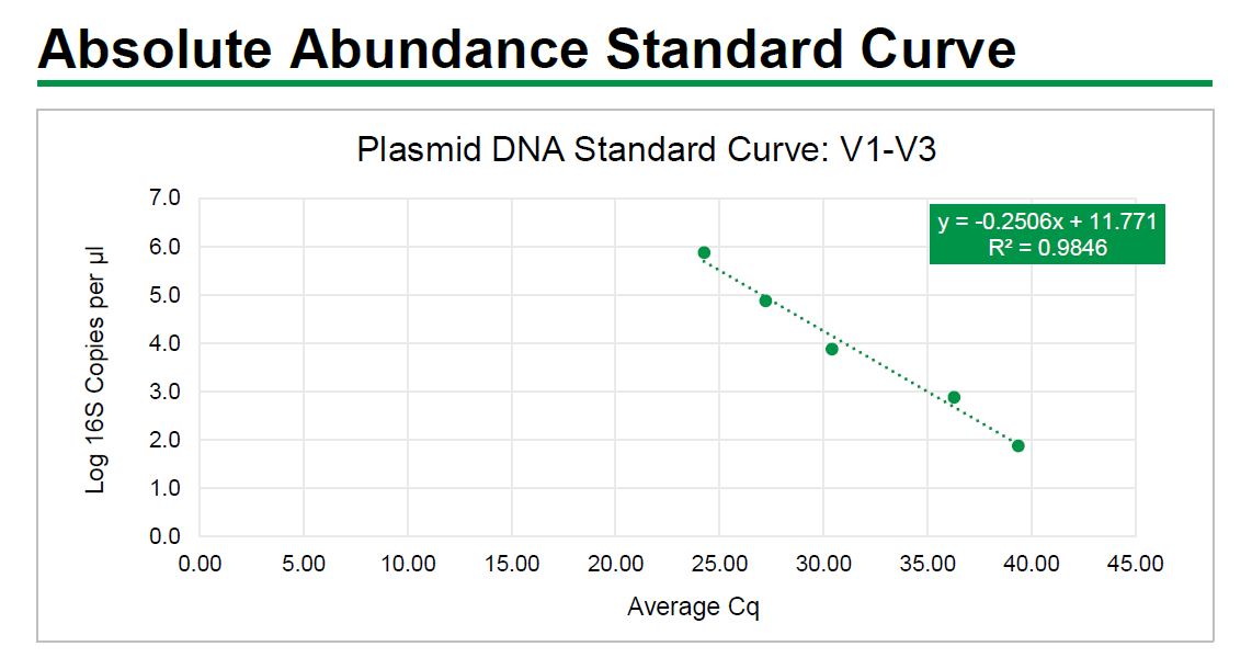
Absolute Abundance Quantification*: A quantitative real-time PCR was set up with a
standard curve. The standard curve was made with plasmid DNA containing one copy
of the 16S gene and one copy of the fungal ITS2 region prepared in 10-fold serial
dilutions. The primers used were the same as those used in Targeted Library
Preparation. The equation generated by the plasmid DNA standard curve was used to
calculate the number of gene copies in the reaction for each sample. The PCR input
volume (2 µl) was used to calculate the number of gene copies per microliter in each
DNA sample.
The number of genome copies per microliter DNA sample was calculated by dividing
the gene copy number by an assumed number of gene copies per genome. The value
used for 16S copies per genome is 4. The value used for ITS copies per genome is 200.
The amount of DNA per microliter DNA sample was calculated using an assumed
genome size of 4.64 x 10⁶ bp, the genome size of Escherichia coli, for 16S samples, or
an assumed genome size of 1.20 x 10⁷ bp, the genome size of Saccharomyces
cerevisiae, for ITS samples. This calculation is shown below:
Calculated Total DNA = Calculated Total Genome Copies × Assumed Genome Size (4.64 × 10⁶ bp) ×
Average Molecular Weight of a DNA bp (660 g/mole/bp) ÷ Avogadro’s Number (6.022 x 10²³/mole)
* Absolute Abundance Quantification is only available for 16S and ITS analyses.
The absolute abundance standard curve data can be viewed in Excel here:
The absolute abundance standard curve is shown below:
The complete report of your project, including all links in this report, can be downloaded by clicking the link provided below. The downloaded file is a compressed ZIP file and once unzipped, open the file “REPORT.html” (may only shown as "REPORT" in your computer) by double clicking it. Your default web browser will open it and you will see the exact content of this report.
Please download and save the file to your computer storage device. The download link will expire after 60 days upon your receiving of this report.
Complete report download link:
To view the report, please follow the following steps:
1.
Download the .zip file from the report link above.
2.
Extract all the contents of the downloaded .zip file to your desktop.
3.
Open the extracted folder and find the "REPORT.html" (may shown as only "REPORT").
4.
Open (double-clicking) the REPORT.html file. Your default browser will open the top age of the complete report. Within the
report, there are links to view all the analyses performed for the project.
The raw NGS sequence data is available for download with the link provided below. The data is a compressed ZIP file and can be unzipped to individual sequence files.
Since this is a Pac-Bio full-length (V1V9) 16S rRNA amplicon sequencing, raw sequences are available for download in a single compressed zip file in the download link below.
After unzipping, you will find individual sequence files for each of your samples with the file extension “*.fastq.gz”.
The files are in FASTQ format and are compressed. FASTQ format is a text-based data format for storing both a biological sequence
and its corresponding quality scores. Most sequence analysis software will be able to open them.
The Sample IDs associated with the fastq files are listed in the table below:
Sample ID
Original Sample ID
Read 1 File Name
Read 2 File Name
F29493.S10
original sample ID here
zr29493_10V1V3_R1.fastq.gz
zr29493_10V1V3_R2.fastq.gz
F29493.S11
original sample ID here
zr29493_11V1V3_R1.fastq.gz
zr29493_11V1V3_R2.fastq.gz
F29493.S12
original sample ID here
zr29493_12V1V3_R1.fastq.gz
zr29493_12V1V3_R2.fastq.gz
F29493.S01
original sample ID here
zr29493_1V1V3_R1.fastq.gz
zr29493_1V1V3_R2.fastq.gz
F29493.S02
original sample ID here
zr29493_2V1V3_R1.fastq.gz
zr29493_2V1V3_R2.fastq.gz
F29493.S03
original sample ID here
zr29493_3V1V3_R1.fastq.gz
zr29493_3V1V3_R2.fastq.gz
F29493.S04
original sample ID here
zr29493_4V1V3_R1.fastq.gz
zr29493_4V1V3_R2.fastq.gz
F29493.S05
original sample ID here
zr29493_5V1V3_R1.fastq.gz
zr29493_5V1V3_R2.fastq.gz
F29493.S06
original sample ID here
zr29493_6V1V3_R1.fastq.gz
zr29493_6V1V3_R2.fastq.gz
F29493.S07
original sample ID here
zr29493_7V1V3_R1.fastq.gz
zr29493_7V1V3_R2.fastq.gz
F29493.S08
original sample ID here
zr29493_8V1V3_R1.fastq.gz
zr29493_8V1V3_R2.fastq.gz
F29493.S09
original sample ID here
zr29493_9V1V3_R1.fastq.gz
zr29493_9V1V3_R2.fastq.gz
Please download and save the file to your computer storage device. The download link will expire after 60 days upon your receiving of this report.
DADA2 is a software package that models and corrects Illumina-sequenced amplicon errors [1].
DADA2 infers sample sequences exactly, without coarse-graining into OTUs,
and resolves differences of as little as one nucleotide. DADA2 identified more real variants
and output fewer spurious sequences than other methods.
DADA2’s advantage is that it uses more of the data. The DADA2 error model incorporates quality information,
which is ignored by all other methods after filtering. The DADA2 error model incorporates quantitative abundances,
whereas most other methods use abundance ranks if they use abundance at all.
The DADA2 error model identifies the differences between sequences, eg. A->C,
whereas other methods merely count the mismatches. DADA2 can parameterize its error model from the data itself,
rather than relying on previous datasets that may or may not reflect the PCR and sequencing protocols used in your study.
Callahan BJ, McMurdie PJ, Rosen MJ, Han AW, Johnson AJ, Holmes SP. DADA2: High-resolution sample inference from Illumina amplicon data. Nat Methods. 2016 Jul;13(7):581-3. doi: 10.1038/nmeth.3869. Epub 2016 May 23. PMID: 27214047; PMCID: PMC4927377.
Analysis Procedures:
DADA2 pipeline includes several tools for read quality control, including quality filtering, trimming, denoising, pair merging and chimera filtering. Below are the major processing steps of DADA2:
Step 1. Read trimming based on sequence quality
The quality of NGS Illumina sequences often decreases toward the end of the reads.
DADA2 allows to trim off the poor quality read ends in order to improve the error
model building and pair mergicing performance.
Step 2. Learn the Error Rates
The DADA2 algorithm makes use of a parametric error model (err) and every
amplicon dataset has a different set of error rates. The learnErrors method
learns this error model from the data, by alternating estimation of the error
rates and inference of sample composition until they converge on a jointly
consistent solution. As in many machine-learning problems, the algorithm must
begin with an initial guess, for which the maximum possible error rates in
this data are used (the error rates if only the most abundant sequence is
correct and all the rest are errors).
Step 3. Infer amplicon sequence variants (ASVs) based on the error model built in previous step. This step is also called sequence "denoising".
The outcome of this step is a list of ASVs that are the equivalent of oligonucleotides.
Step 4. Merge paired reads. If the sequencing products are read pairs, DADA2 will merge the R1 and R2 ASVs into single sequences.
Merging is performed by aligning the denoised forward reads with the reverse-complement of the corresponding
denoised reverse reads, and then constructing the merged “contig” sequences.
By default, merged sequences are only output if the forward and reverse reads overlap by
at least 12 bases, and are identical to each other in the overlap region (but these conditions can be changed via function arguments).
Step 5. Remove chimera.
The core dada method corrects substitution and indel errors, but chimeras remain. Fortunately, the accuracy of sequence variants
after denoising makes identifying chimeric ASVs simpler than when dealing with fuzzy OTUs.
Chimeric sequences are identified if they can be exactly reconstructed by
combining a left-segment and a right-segment from two more abundant “parent” sequences. The frequency of chimeric sequences varies substantially
from dataset to dataset, and depends on on factors including experimental procedures and sample complexity.
Results
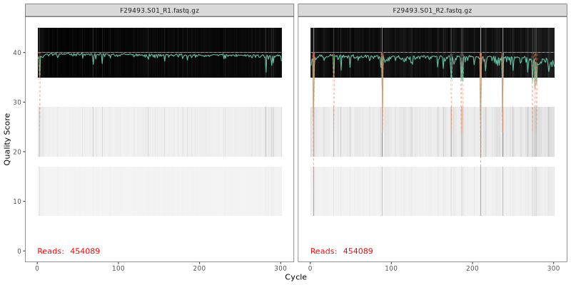
1. Read Quality Plots NGS sequence analaysis starts with visualizing the quality of the sequencing. Below are the quality plots of the first
sample for the R1 and R2 reads separately. In gray-scale is a heat map of the frequency of each quality score at each base position. The mean
quality score at each position is shown by the green line, and the quartiles of the quality score distribution by the orange lines.
The forward reads are usually of better quality. It is a common practice to trim the last few nucleotides to avoid less well-controlled errors
that can arise there. The trimming affects the downstream steps including error model building, merging and chimera calling. FOMC uses an empirical
approach to test many combinations of different trim length in order to achieve best final amplicon sequence variants (ASVs), see the next
section “Optimal trim length for ASVs”.
2. Optimal trim length for ASVs The final number of merged and chimera-filtered ASVs depends on the quality filtering (hence trimming) in the very beginning of the DADA2 pipeline.
In order to achieve highest number of ASVs, an empirical approach was used -
Create a random subset of each sample consisting of 5,000 R1 and 5,000 R2 (to reduce computation time)
Trim 10 bases at a time from the ends of both R1 and R2 up to 50 bases
For each combination of trimmed length (e.g., 300x300, 300x290, 290x290 etc), the trimmed reads are
subject to the entire DADA2 pipeline for chimera-filtered merged ASVs
The combination with highest percentage of the input reads becoming final ASVs is selected for the complete set of data
Below is the result of such operation, showing ASV percentages of total reads for all trimming combinations (1st Column = R1 lengths in bases; 1st Row = R2 lengths in bases):
R1/R2
301
291
281
271
261
251
301
91.44%
91.40%
91.57%
91.51%
91.44%
14.23%
291
91.47%
91.43%
91.61%
91.48%
14.26%
11.68%
281
91.47%
91.44%
91.54%
14.31%
11.65%
5.22%
271
91.42%
91.31%
14.24%
11.73%
5.21%
0.37%
261
91.28%
14.22%
11.63%
5.24%
0.37%
0.00%
251
14.28%
11.64%
5.21%
0.37%
0.00%
0.00%
Based on the above result, the trim length combination of R1 = 291 bases and R2 = 281 bases (highlighted red above), was chosen for generating final ASVs for all sequences.
This combination generated highest number of merged non-chimeric ASVs and was used for downstream analyses, if requested.
3. Error plots from learning the error rates
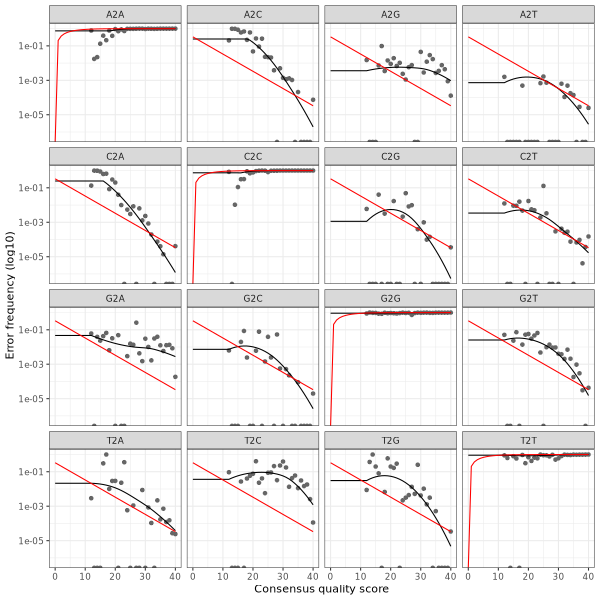
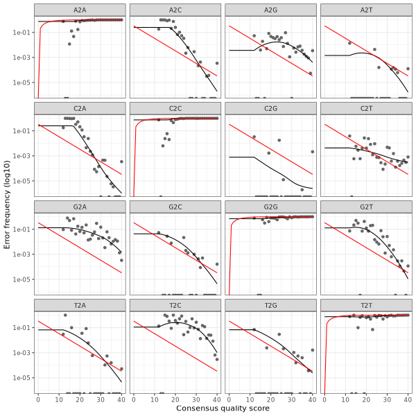
After DADA2 building the error model for the set of data, it is always worthwhile, as a sanity check if nothing else, to visualize the estimated error rates.
The error rates for each possible transition (A→C, A→G, …) are shown below. Points are the observed error rates for each consensus quality score.
The black line shows the estimated error rates after convergence of the machine-learning algorithm.
The red line shows the error rates expected under the nominal definition of the Q-score.
The ideal result would be the estimated error rates (black line) are a good fit to the observed rates (points), and the error rates drop
with increased quality as expected.
Forward Read R1 Error Plot
Reverse Read R2 Error Plot
The PDF version of these plots are available here:
4. DADA2 Result Summary The table below shows the summary of the DADA2 analysis,
tracking paired read counts of each samples for all the steps during DADA2 denoising process -
including end-trimming (filtered), denoising (denoisedF, denoisedF), pair merging (merged) and chimera removal (nonchim).
Sample ID
F29493.S01
F29493.S02
F29493.S03
F29493.S04
F29493.S05
F29493.S06
F29493.S07
F29493.S08
F29493.S09
F29493.S10
F29493.S11
F29493.S12
Row Sum
Percentage
input
454,089
525,523
407,575
407,576
482,310
621,282
408,657
451,137
491,238
503,059
620,972
623,396
5,996,814
100.00%
filtered
454,035
525,460
407,520
407,537
482,268
621,207
408,597
451,084
491,181
502,991
620,894
623,303
5,996,077
99.99%
denoisedF
453,417
524,478
406,086
406,180
481,551
619,083
406,519
449,402
490,306
502,265
619,840
621,818
5,980,945
99.74%
denoisedR
449,685
520,068
403,127
403,332
477,805
615,182
404,358
446,618
486,352
497,974
614,572
617,126
5,936,199
98.99%
merged
443,406
513,390
395,901
395,840
471,117
604,092
396,793
438,685
479,073
490,678
605,669
606,928
5,841,572
97.41%
nonchim
433,415
493,972
345,176
355,377
465,445
527,379
341,898
384,857
464,712
479,691
588,370
555,931
5,436,223
90.65%
This table can be downloaded as an Excel table below:
5. DADA2 Amplicon Sequence Variants (ASVs). A total of 555 unique merged and chimera-free ASV sequences were identified, and their corresponding
read counts for each sample are available in the "ASV Read Count Table" with rows for the ASV sequences and columns for sample. This read count table can be used for
microbial profile comparison among different samples and the sequences provided in the table can be used to taxonomy assignment.
The species-level, open-reference 16S rRNA NGS reads taxonomy assignment pipeline
Version 20210310a
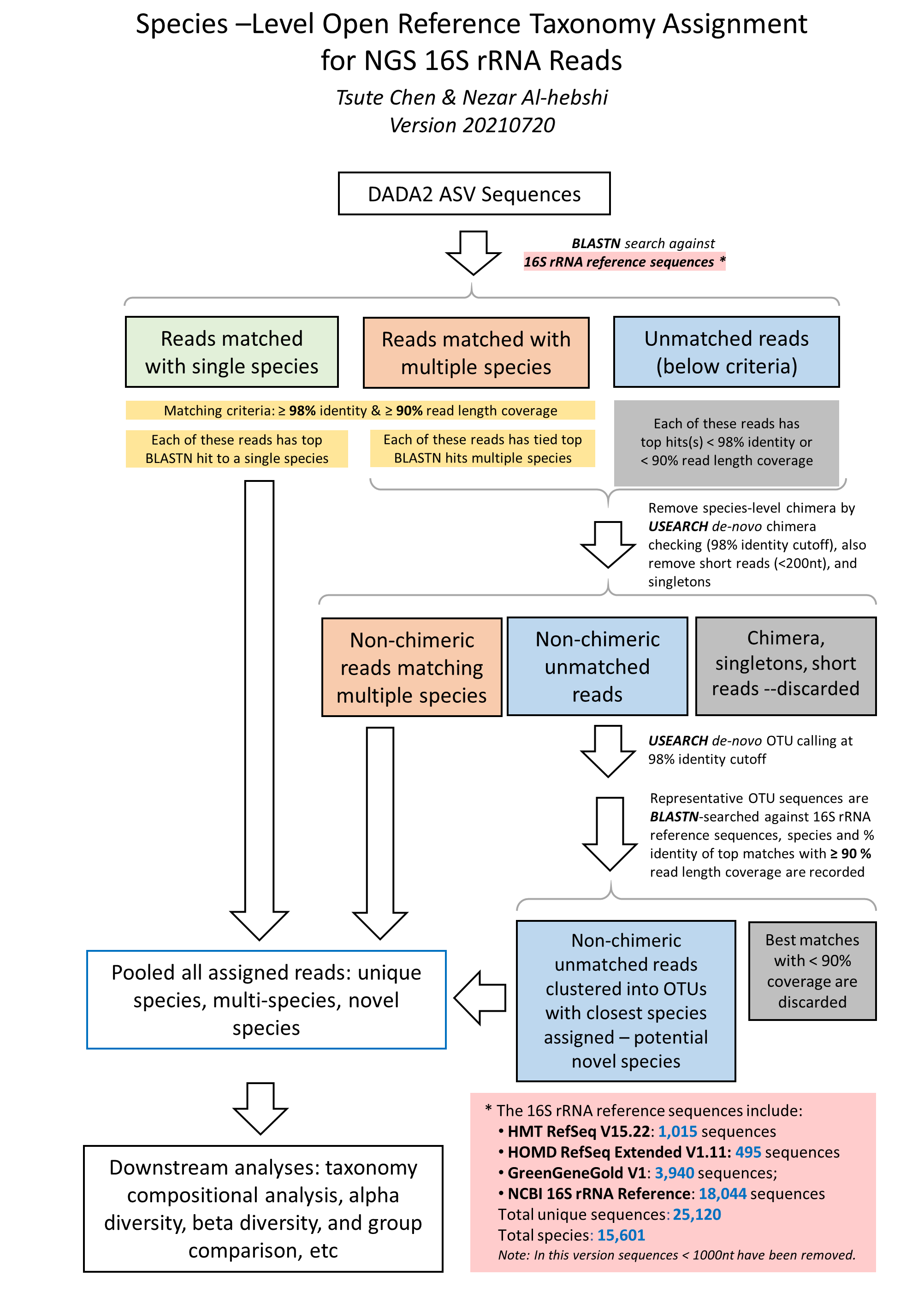
The close-reference taxonomy assignment of the ASV sequences using BLASTN is based on the algorithm published by Al-Hebshi et. al. (2015)[2].
1. Raw sequences reads in FASTA format were BLASTN-searched against a combined set of 16S rRNA reference sequences - the FOMC 16S rRNA Reference Sequences version 20221029 (https://microbiome.forsyth.org/ftp/refseq/).
This set consists of the HOMD (version 15.22 http://www.homd.org/index.php?name=seqDownload&file&type=R ), Mouse Oral Microbiome Database (MOMD version 5.1 https://momd.org/ftp/16S_rRNA_refseq/MOMD_16S_rRNA_RefSeq/V5.1/),
and the NCBI 16S rRNA reference sequence set (https://ftp.ncbi.nlm.nih.gov/blast/db/16S_ribosomal_RNA.tar.gz).
These sequences were screened and combined to remove short sequences (<1000nt), chimera, duplicated and sub-sequences,
as well as sequences with poor taxonomy annotation (e.g., without species information).
This process resulted in 1,015 full-length 16S rRNA sequences from HOMD V15.22, 356 from MOMD V5.1, and 22,126 from NCBI, a total of 23,497 sequences.
Altogether these sequence represent a total of 17,035 oral and non-oral microbial species.
The NCBI BLASTN version 2.7.1+ (Zhang et al, 2000) [3] was used with the default parameters.
Reads with ≥ 98% sequence identity to the matched reference and ≥ 90% alignment length
(i.e., ≥ 90% of the read length that was aligned to the reference and was used to calculate
the sequence percent identity) were classified based on the taxonomy of the reference sequence
with highest sequence identity. If a read matched with reference sequences representing
more than one species with equal percent identity and alignment length, it was subject
to chimera checking with USEARCH program version v8.1.1861 (Edgar 2010). Non-chimeric reads with multi-species
best hits were considered valid and were assigned with a unique species
notation (e.g., spp) denoting unresolvable multiple species.
2. Unassigned reads (i.e., reads with < 98% identity or < 90% alignment length) were pooled together and reads < 200 bases were
removed. The remaining reads were subject to the de novo
operational taxonomy unit (OTU) calling and chimera checking using the USEARCH program version v8.1.1861 (Edgar 2010)[4].
The de novo OTU calling and chimera checking was done using 98% as the sequence identity cutoff, i.e., the species-level OTU.
The output of this step produced species-level de novo clustered OTUs with 98% identity.
Representative reads from each of the OTUs/species were then BLASTN-searched
against the same reference sequence set again to determine the closest species for
these potential novel species. These potential novel species were pooled together with the reads that were signed to specie-level in
the previous step, for down-stream analyses.
Reference:
Al-Hebshi NN, Nasher AT, Idris AM, Chen T. Robust species taxonomy assignment algorithm for 16S rRNA NGS reads: application
to oral carcinoma samples. J Oral Microbiol. 2015 Sep 29;7:28934. doi: 10.3402/jom.v7.28934. PMID: 26426306; PMCID: PMC4590409.
Zhang Z, Schwartz S, Wagner L, Miller W. A greedy algorithm for aligning DNA sequences. J Comput Biol. 2000 Feb-Apr;7(1-2):203-14. doi: 10.1089/10665270050081478. PMID: 10890397.
Edgar RC. Search and clustering orders of magnitude faster than BLAST.
Bioinformatics. 2010 Oct 1;26(19):2460-1. doi: 10.1093/bioinformatics/btq461. Epub 2010 Aug 12. PubMed PMID: 20709691.
3. Designations used in the taxonomy:
	1) Taxonomy levels are indicated by these prefixes:

	   k__: domain/kingdom
	   p__: phylum
	   c__: class
	   o__: order
	   f__: family
	   g__: genus
	   s__: species

	   Example:

	   k__Bacteria;p__Firmicutes;c__Clostridia;o__Clostridiales;f__Lachnospiraceae;g__Blautia;s__faecis

	2) Unique level identified – known species:

	   k__Bacteria;p__Firmicutes;c__Clostridia;o__Clostridiales;f__Lachnospiraceae;g__Roseburia;s__hominis

	   The above example shows some reads match to a single species (all levels are unique)

	3) Non-unique level identified – known species:

	   k__Bacteria;p__Firmicutes;c__Clostridia;o__Clostridiales;f__Lachnospiraceae;g__Roseburia;s__multispecies_spp123_3

	   The above example “s__multispecies_spp123_3” indicates certain reads equally match to 3 species of the
	   genus Roseburia; the “spp123” is a temporally assigned species ID.

	   k__Bacteria;p__Firmicutes;c__Clostridia;o__Clostridiales;f__Lachnospiraceae;g__multigenus;s__multispecies_spp234_5

	   The above example indicates certain reads match equally to 5 different species, which belong to multiple genera.;
	   the “spp234” is a temporally assigned species ID.

	4) Unique level identified – unknown species, potential novel species:

	   k__Bacteria;p__Firmicutes;c__Clostridia;o__Clostridiales;f__Lachnospiraceae;g__Roseburia;s__ hominis_nov_97%

	   The above example indicates that some reads have no match to any of the reference sequences with
	   sequence identity ≥ 98% and percent coverage (alignment length)  ≥ 98% as well. However this groups
	   of reads (actually the representative read from a de novo  OTU) has 96% percent identity to
	   Roseburia hominis, thus this is a potential novel species, closest to Roseburia hominis.
	   (But they are not the same species).

	5) Multiple level identified – unknown species, potential novel species:
	   k__Bacteria;p__Firmicutes;c__Clostridia;o__Clostridiales;f__Lachnospiraceae;g__Roseburia;s__ multispecies_sppn123_3_nov_96%

	   The above example indicates that some reads have no match to any of the reference sequences
	   with sequence identity ≥ 98% and percent coverage (alignment length)  ≥ 98% as well.
	   However this groups of reads (actually the representative read from a de novo  OTU)
	   has 96% percent identity equally to 3 species in Roseburia. Thus this is no single
	   closest species, instead this group of reads match equally to multiple species at 96%.
	   Since they have passed chimera check so they represent a novel species. “sppn123” is a
	   temporary ID for this potential novel species.
4. The taxonomy assignment algorithm is illustrated in this flow char below:
Read Taxonomy Assignment - Result Summary *
Code
Category
MPC=0% (>=1 read)
MPC=0.01%(>=0 reads)
A
Total reads
5,436,223
5,436,223
B
Total assigned reads
5,433,964
5,433,964
C
Assigned reads in species with read count < MPC
0
0
D
Assigned reads in samples with read count < 500
0
0
E
Total samples
12
12
F
Samples with reads >= 500
12
12
G
Samples with reads < 500
0
0
H
Total assigned reads used for analysis (B-C-D)
5,433,964
5,433,964
I
Reads assigned to single species
5,252,089
5,252,089
J
Reads assigned to multiple species
140,849
140,849
K
Reads assigned to novel species
41,026
41,026
L
Total number of species
201
201
M
Number of single species
52
52
N
Number of multi-species
4
4
O
Number of novel species
145
145
P
Total unassigned reads
2,259
2,259
Q
Chimeric reads
121
121
R
Reads without BLASTN hits
1,306
1,306
S
Others: short, low quality, singletons, etc.
832
832
A=B+P=C+D+H+Q+R+S
E=F+G
B=C+D+H
H=I+J+K
L=M+N+O
P=Q+R+S
* MPC = Minimal percent (of all assigned reads) read count per species, species with read count < MPC were removed.
* Samples with reads < 500 were removed from downstream analyses.
* The assignment result from MPC=0.1% was used in the downstream analyses.
Read Taxonomy Assignment - ASV Species-Level Read Counts Table
This table shows the read counts for each sample (columns) and each species identified based on the ASV sequences.
The downstream analyses were based on this table.
The species listed in the table has full taxonomy and a dynamically assigned species ID specific to this report.
When some reads match with the reference sequences of more than one species equally (i.e., same percent identiy and alignmnet coverage),
they can't be assigned to a particular species. Instead, they are assigned to multiple species with the species notaton
"s__multispecies_spp2_2". In this notation, spp2 is the dynamic ID assigned to these reads that hit multiple sequences and the "_2"
at the end of the notation means there are two species in the spp2.
You can look up which species are included in the multi-species assignment, in this table below:
Another type of notation is "s__multispecies_sppn2_2", in which the "n" in the sppn2 means it's a potential novel species because all the reads in this species
have < 98% idenity to any of the reference sequences. They were grouped together based on de novo OTU clustering at 98% identity cutoff. And then
a representative sequence was chosed to BLASTN search against the reference database to find the closest match (but will still be < 98%). This representative
sequence also matched equally to more than one species, hence the "spp" was given in the label.
In ecology, alpha diversity (α-diversity) is the mean species diversity in sites or habitats at a local scale.
The term was introduced by R. H. Whittaker[5][6] together with the terms beta diversity (β-diversity)
and gamma diversity (γ-diversity). Whittaker's idea was that the total species diversity in a landscape
(gamma diversity) is determined by two different things, the mean species diversity in sites or habitats
at a more local scale (alpha diversity) and the differentiation among those habitats (beta diversity).
Diversity measures are affected by the sampling depth. Rarefaction is a technique to assess species richness from the results of sampling. Rarefaction allows
the calculation of species richness for a given number of individual samples, based on the construction
of so-called rarefaction curves. This curve is a plot of the number of species as a function of the
number of samples. Rarefaction curves generally grow rapidly at first, as the most common species are found,
but the curves plateau as only the rarest species remain to be sampled [7].
The two main factors taken into account when measuring diversity are richness and evenness.
Richness is a measure of the number of different kinds of organisms present in a particular area.
Evenness compares the similarity of the population size of each of the species present. There are
many different ways to measure the richness and evenness. These measurements are called "estimators" or "indices".
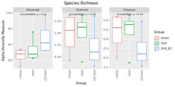
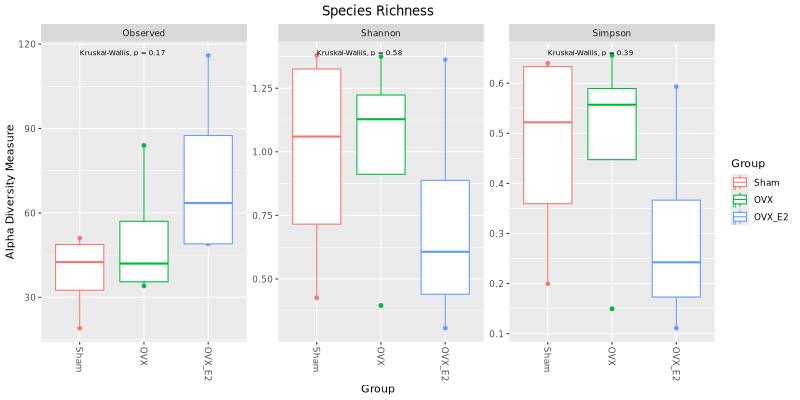
Below is a diversity of 3 commonly used indices showing the values for all the samples (dots) and in groups (boxes) at the species level.
Printed on each graph is the statistical significance p values of the difference between the groups.
The significance is calculated using either Kruskal-Wallis test or the Wilcoxon rank sum test, both are non-parametric methods (since
microbiome read count data are considered non-normally distributed) for testing
whether samples originate from the same distribution (i.e., no difference between groups). The Kruskal-Wallis test is used to compare three or more
independent groups to determine if there are statistically significant differences between their medians. The Wilcoxon Rank Sum test, also known as
the Mann-Whitney U test, is used to compare two independent groups to determine if there is a significant difference between their distributions.
The p-value is shown on the top of each graph. A p-value < 0.05 is considered statistically significant between/among the test groups.
Alpha Diversity Box Plots for All Groups - Species Level
Alpha Diversity Box Plots for Individual Comparisons at Species level
Beta diversity compares the similarity (or dissimilarity) of microbial profiles between different
groups of samples. There are many different similarity/dissimilarity metrics [8].
In general, they can be quantitative (using sequence abundance, e.g., Bray-Curtis or weighted UniFrac)
or binary (considering only presence-absence of sequences, e.g., binary Jaccard or unweighted UniFrac).
They can be even based on phylogeny (e.g., UniFrac metrics) or not (non-UniFrac metrics, such as Bray-Curtis, etc.).
For microbiome studies, species profiles of samples can be compared with the Bray-Curtis dissimilarity,
which is based on the count data type. The pair-wise Bray-Curtis dissimilarity matrix of all samples can then be
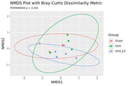
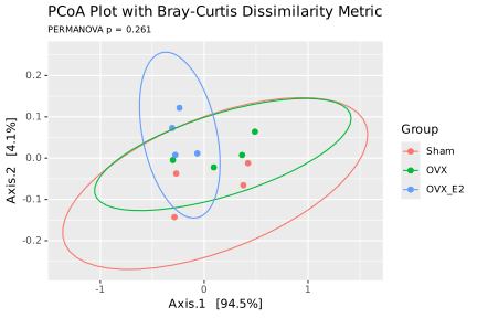
subject to either multi-dimensional scaling (MDS, also known as PCoA) or non-metric MDS (NMDS).
MDS/PCoA is a
scaling or ordination method that starts with a matrix of similarities or dissimilarities
between a set of samples and aims to produce a low-dimensional graphical plot of the data
in such a way that distances between points in the plot are close to original dissimilarities.
NMDS is similar to MDS, however it does not use the dissimilarities data, instead it converts them into
the ranks and use these ranks in the calculation.
In our beta diversity analysis, Bray-Curtis dissimilarity matrix was first calculated and then plotted by the PCoA and
NMDS separately. Below are beta diveristy results for all groups together, at the Species level:
NMDS and PCoA Plots for All Groups - Species Level
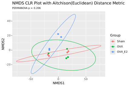
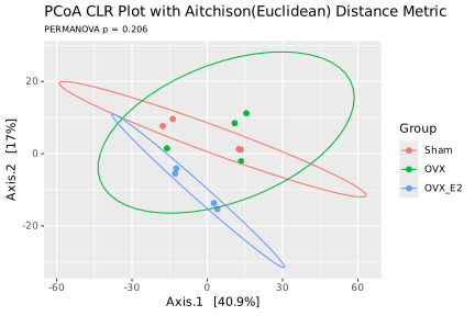
The above PCoA and NMDS plots are based on count data. The count data can also be transformed into centered log ratio (CLR)
for each species. The CLR data is no longer count data and cannot be used in Bray-Curtis dissimilarity calculation. Instead
CLR can be compared with Euclidean distances. When CLR data are compared by Euclidean distance, the distance is also called
Aitchison distance.
Below are the NMDS and PCoA plots of the Aitchison distances of the samples at the Species level:
NMDS and PCoA Plots for Individual Comparisons at Species level
16S rRNA next generation sequencing (NGS) generates a fixed number of reads that reflect the proportion of different
species in a sample, i.e., the relative abundance of species, instead of the absolute abundance.
In Mathematics, measurements involving probabilities, proportions, percentages, and ppm can all
be thought of as compositional data. This makes the microbiome read count data “compositional”
(Gloor et al, 2017). In general, compositional data represent parts of a whole which only
carry relative information [9].
The problem of microbiome data being compositional arises when comparing two groups of samples for
identifying “differentially abundant” species. A species with the same absolute abundance between two
conditions, its relative abundances in the two conditions (e.g., percent abundance) can become different
if the relative abundance of other species change greatly. This problem can lead to incorrect conclusion
in terms of differential abundance for microbial species in the samples.
When studying differential abundance (DA), the current better approach is to transform the read count
data into log ratio data. The ratios are calculated between read counts of all species in a sample to
a “reference” count (e.g., mean read count of the sample). The log ratio data allow the detection of DA
species without being affected by percentage bias mentioned above
In this report, a compositional DA analysis tool “ANCOM” (analysis of composition of microbiomes)
was used [10]. ANCOM transforms the count data into log-ratios and thus is more suitable for comparing
the composition of microbiomes in two or more populations. "ANCOM" generates a table of features with
W-statistics and whether the null hypothesis is rejected. The “W” is the W-statistic, or number of
features that a single feature is tested to be significantly different against. Hence the higher the "W"
the more statistical sifgnificant that a feature/species is differentially abundant.
References:
Gloor GB, Macklaim JM, Pawlowsky-Glahn V, Egozcue JJ. Microbiome Datasets Are Compositional: And This Is Not Optional. Front Microbiol.
2017 Nov 15;8:2224. doi: 10.3389/fmicb.2017.02224. PMID: 29187837; PMCID: PMC5695134.
Mandal S, Van Treuren W, White RA, Eggesbø M, Knight R, Peddada SD. Analysis of composition of
microbiomes: a novel method for studying microbial composition. Microb Ecol Health Dis.
2015 May 29;26:27663. doi: 10.3402/mehd.v26.27663. PMID: 26028277; PMCID: PMC4450248.
Starting with version V1.2, we include the results of ANCOM-BC (Analysis of Compositions of
Microbiomes with Bias Correction) (Lin and Peddada 2020) [11]. ANCOM-BC is an updated version of "ANCOM" that:
(a) provides statistically valid test with appropriate p-values,
(b) provides confidence intervals for differential abundance of each taxon,
(c) controls the False Discovery Rate (FDR),
(d) maintains adequate power, and
(e) is computationally simple to implement.
The bias correction (BC) addresses a challenging problem of the bias introduced by differences in
the sampling fractions across samples. This bias has been a major hurdle in performing DA analysis of microbiome data.
ANCOM-BC estimates the unknown sampling fractions and corrects the bias induced by their differences among samples.
The absolute abundance data are modeled using a linear regression framework.
Starting with version V1.43, ANCOM-BC2 is used instead of ANCOM-BC, So that multiple pairwise directional test can be performed (if there are more than two gorups in a comparison).
When performing pairwise directional test, the mixed directional false discover rate (mdFDR) is taken into account. The mdFDR
is the combination of false discovery rate due to multiple testing, multiple pairwise comparisons, and directional tests within
each pairwise comparison. The mdFDR is adopted from (Guo, Sarkar, and Peddada 2010 [12]; Grandhi, Guo, and Peddada 2016 [13]). For more detail
explanation and additional features of ANCOM-BC2 please see author's documentation.
References:
Lin H, Peddada SD. Analysis of compositions of microbiomes with bias correction.
Nat Commun. 2020 Jul 14;11(1):3514. doi: 10.1038/s41467-020-17041-7.
PMID: 32665548; PMCID: PMC7360769.
Guo W, Sarkar SK, Peddada SD. Controlling false discoveries in multidimensional directional decisions, with applications to gene expression data on ordered categories. Biometrics. 2010 Jun;66(2):485-92. doi: 10.1111/j.1541-0420.2009.01292.x. Epub 2009 Jul 23. PMID: 19645703; PMCID: PMC2895927.
Grandhi A, Guo W, Peddada SD. A multiple testing procedure for multi-dimensional pairwise comparisons with application to gene expression studies. BMC Bioinformatics. 2016 Feb 25;17:104. doi: 10.1186/s12859-016-0937-5. PMID: 26917217; PMCID: PMC4768411.
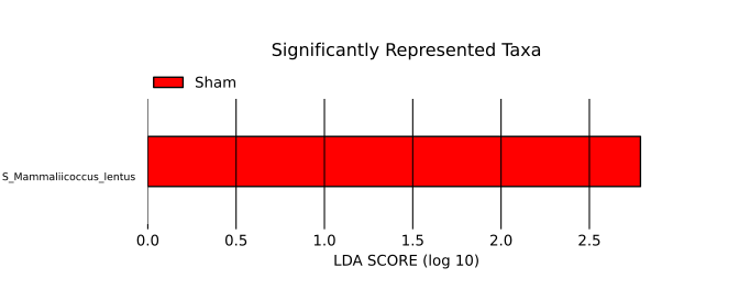
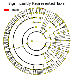
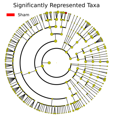
LEfSe (Linear Discriminant Analysis Effect Size) is an alternative method to find "organisms, genes, or
pathways that consistently explain the differences between two or more microbial communities" (Segata et al., 2011) [14].
Specifically, LEfSe uses rank-based Kruskal-Wallis (KW) sum-rank test to detect features with significant
differential (relative) abundance with respect to the class of interest. Since it is rank-based, instead of proportional based,
the differential species identified among the comparison groups is less biased (than percent abundance based).
Reference:
Segata N, Izard J, Waldron L, Gevers D, Miropolsky L, Garrett WS, Huttenhower C. Metagenomic biomarker discovery and explanation. Genome Biol. 2011 Jun 24;12(6):R60. doi: 10.1186/gb-2011-12-6-r60. PMID: 21702898; PMCID: PMC3218848.
To analyze the co-occurrence or co-exclusion between microbial species among different samples, network correlation
analysis tools are usually used for this purpose. However, microbiome count data are compositional. If count data are normalized to the total number of counts in the
sample, the data become not independent and traditional statistical metrics (e.g., correlation) for the detection
of specie-species relationships can lead to spurious results. In addition, sequencing-based studies typically
measure hundreds of OTUs (species) on few samples; thus, inference of OTU-OTU association networks is severely
under-powered. We provide the network association result with SparCC (Sparse Correlations for Compositional data)(Friedman & Alm 2012), which
is a method for inferring correlations from compositional data. SparCC estimates the linear Pearson correlations between
the log-transformed components.
The results of this analysis are for research purpose only. They are not intended to diagnose, treat, cure, or prevent any disease. Forsyth and FOMC
are not responsible for use of information provided in this report outside the research area.