FOMC Service Report

16S rRNA Gene V1V3 Amplicon Sequencing

Version V1.41 fork

Version History

The Forsyth Institute, Cambridge, MA, USA
October 19, 2023

Project ID: 20231018_oral_w8


I. Project Summary

Project 20231018_oral_w8 services do not include NGS sequencing of the V1V3 region of the 16S rRNA gene amplicons from the samples. First and foremost, please download this report. These links will expire after 60 days. We cannot guarantee the availability of your data after 60 days.

Full Bioinformatics analysis service was requested.

We provide many downstream analyses such as taxonomy assignment, alpha and beta diversity analyses, and differential abundance analysis.

For taxonomy assignment, most informative would be the taxonomy barplots. We provide an interactive barplots to show the relative abundance of microbes at different taxonomy levels (from Phylum to species) that you can choose.

If you specify which groups of samples you want to compare for differential abundance, we provide both ANCOM and LEfSe differential abundance analysis.


II. Workflow Checklist

1.Sample Received
2.Sample Quality Evaluated
3.Sample Prepared for Sequencing
4.Next-Gen Sequencing
5.Sequence Quality Check
6.Absolute Abundance
7.Report and Raw Sequence Data Available for Download
8.Bioinformatics Analysis - Reads Processing (DADA2 Quality Trimming, Denoising, Paired Reads Merging)
9.Bioinformatics Analysis - Reads Taxonomy Assignment
10.Bioinformatics Analysis - Alpha Diversity Analysis
11.Bioinformatics Analysis - Beta Diversity Analysis
12.Bioinformatics Analysis - Differential Abundance Analysis
13.Bioinformatics Analysis - Heatmap Profile
14.Bioinformatics Analysis - Network Association
 

III. NGS Sequencing

Not available
 

IV. Complete Report Download

The complete report of your project, including all links in this report, can be downloaded by clicking the link provided below. The downloaded file is a compressed ZIP file and once unzipped, open the file “REPORT.html” (may only shown as "REPORT" in your computer) by double clicking it. Your default web browser will open it and you will see the exact content of this report.

Please download and save the file to your computer storage device. The download link will expire after 60 days upon your receiving of this report.

Complete report download link:

To view the report, please follow the following steps:
1.Download the .zip file from the report link above.
2.Extract all the contents of the downloaded .zip file to your desktop.
3.Open the extracted folder and find the "REPORT.html" (may shown as only "REPORT").
4.Open (double-clicking) the REPORT.html file. Your default browser will open the top age of the complete report. Within the report, there are links to view all the analyses performed for the project.


V. Raw Sequence Data Download

Not available
 

VI. Analysis - DADA2 Read Processing

Not available
 

Sample Meta Information

#SampleIDGenderGroup_1Group_2Group
O13FCMCTaconicF CMC Taconic
O14FCMCTaconicF CMC Taconic
O15FCMCTaconicF CMC Taconic
O16FCMCTaconicF CMC Taconic
O17FCMCTaconicF CMC Taconic
O18FCMCTaconicF CMC Taconic
O19FCMCTaconicF CMC Taconic
O20FCMCTaconicF CMC Taconic
O21MCMCTaconicM CMC Taconic
O22MCMCTaconicM CMC Taconic
O23MCMCTaconicM CMC Taconic
O24MCMCTaconicM CMC Taconic
O25MCMCTaconicM CMC Taconic
O26MCMCTaconicM CMC Taconic
O27MCMCTaconicM CMC Taconic
O28MCMCTaconicM CMC Taconic
O29FS_mitisTaconicF S_mitis Taconic
O30FS_mitisTaconicF S_mitis Taconic
O31FS_mitisTaconicF S_mitis Taconic
O32FS_mitisTaconicF S_mitis Taconic
O33FS_mitisTaconicF S_mitis Taconic
O34FS_mitisTaconicF S_mitis Taconic
O35FS_mitisTaconicF S_mitis Taconic
O36FS_mitisTaconicF S_mitis Taconic
O37MS_mitisTaconicM S_mitis Taconic
O38MS_mitisTaconicM S_mitis Taconic
O39MS_mitisTaconicM S_mitis Taconic
O40MS_mitisTaconicM S_mitis Taconic
O41MS_mitisTaconicM S_mitis Taconic
O42MS_mitisTaconicM S_mitis Taconic
O43MS_mitisTaconicM S_mitis Taconic
O44MS_mitisTaconicM S_mitis Taconic
O57FCMCJacksonF CMC Jackson
O58FCMCJacksonF CMC Jackson
O59FCMCJacksonF CMC Jackson
O60FCMCJacksonF CMC Jackson
O61FCMCJacksonF CMC Jackson
O62FCMCJacksonF CMC Jackson
O63FCMCJacksonF CMC Jackson
O64FCMCJacksonF CMC Jackson
O65MCMCJacksonM CMC Jackson
O66MCMCJacksonM CMC Jackson
O67MCMCJacksonM CMC Jackson
O68MCMCJacksonM CMC Jackson
O69MCMCJacksonM CMC Jackson
O70MCMCJacksonM CMC Jackson
O71MCMCJacksonM CMC Jackson
O72MCMCJacksonM CMC Jackson
O73FS_mitisJacksonF S_mitis Jackson
O74FS_mitisJacksonF S_mitis Jackson
O75FS_mitisJacksonF S_mitis Jackson
O76FS_mitisJacksonF S_mitis Jackson
O77FS_mitisJacksonF S_mitis Jackson
O78FS_mitisJacksonF S_mitis Jackson
O79FS_mitisJacksonF S_mitis Jackson
O80FS_mitisJacksonF S_mitis Jackson
O81MS_mitisJacksonM S_mitis Jackson
O82MS_mitisJacksonM S_mitis Jackson
O83MS_mitisJacksonM S_mitis Jackson
O84MS_mitisJacksonM S_mitis Jackson
O85MS_mitisJacksonM S_mitis Jackson
O86MS_mitisJacksonM S_mitis Jackson
O87MS_mitisJacksonM S_mitis Jackson
O88MS_mitisJacksonM S_mitis Jackson
N1NegativeNegativeNegativeNegative Negative Negative
N2NegativeNegativeNegativeNegative Negative Negative
N3NegativeNegativeNegativeNegative Negative Negative
N4NegativeNegativeNegativeNegative Negative Negative
N5NegativeNegativeNegativeNegative Negative Negative
N6NegativeNegativeNegativeNegative Negative Negative
N7NegativeNegativeNegativeNegative Negative Negative
N8NegativeNegativeNegativeNegative Negative Negative
N9NegativeNegativeNegativeNegative Negative Negative
N10NegativeNegativeNegativeNegative Negative Negative
N11NegativeNegativeNegativeNegative Negative Negative
N12NegativeNegativeNegativeNegative Negative Negative
N13NegativeNegativeNegativeNegative Negative Negative
N14NegativeNegativeNegativeNegative Negative Negative
N15NegativeNegativeNegativeNegative Negative Negative
N16NegativeNegativeNegativeNegative Negative Negative
N17NegativeNegativeNegativeNegative Negative Negative
P1PositivePositivePositivePositive Positive Positive


ASV Read Counts by Samples

#Sample IDRead Count
N23,015
N314,565
N122,164
P131,399
O2648,940
N452,365
N853,975
N756,381
N661,322
O4364,876
O1866,414
N586,220
O4088,040
O2795,521
O15100,981
O61101,944
N9101,958
O19104,322
O88105,669
O36106,010
O80107,550
O76111,281
O28111,912
O22112,853
O83114,114
O41115,224
O84117,557
O16119,653
O20119,725
O38119,965
O78120,570
O66121,783
O75126,428
O79129,712
O77131,439
O23135,965
O30136,638
O69138,214
O33139,360
O31139,699
O42140,224
O72141,512
O87147,371
O21147,941
O14150,212
O86151,365
O82152,139
O25152,186
O67152,309
O17157,670
O74160,444
O24163,954
O37164,488
O81164,604
O73167,250
O39168,830
O71169,098
O68170,319
O65175,480
O85178,334
O70179,070
O34182,734
O32187,363
O44197,449
O29197,627
O35201,358
O63210,518
O60220,065
O62222,518
O13223,279
O57229,108
O58245,567
O64254,363
O59254,735


VII. Analysis - Read Taxonomy Assignment

Read Taxonomy Assignment - Methods


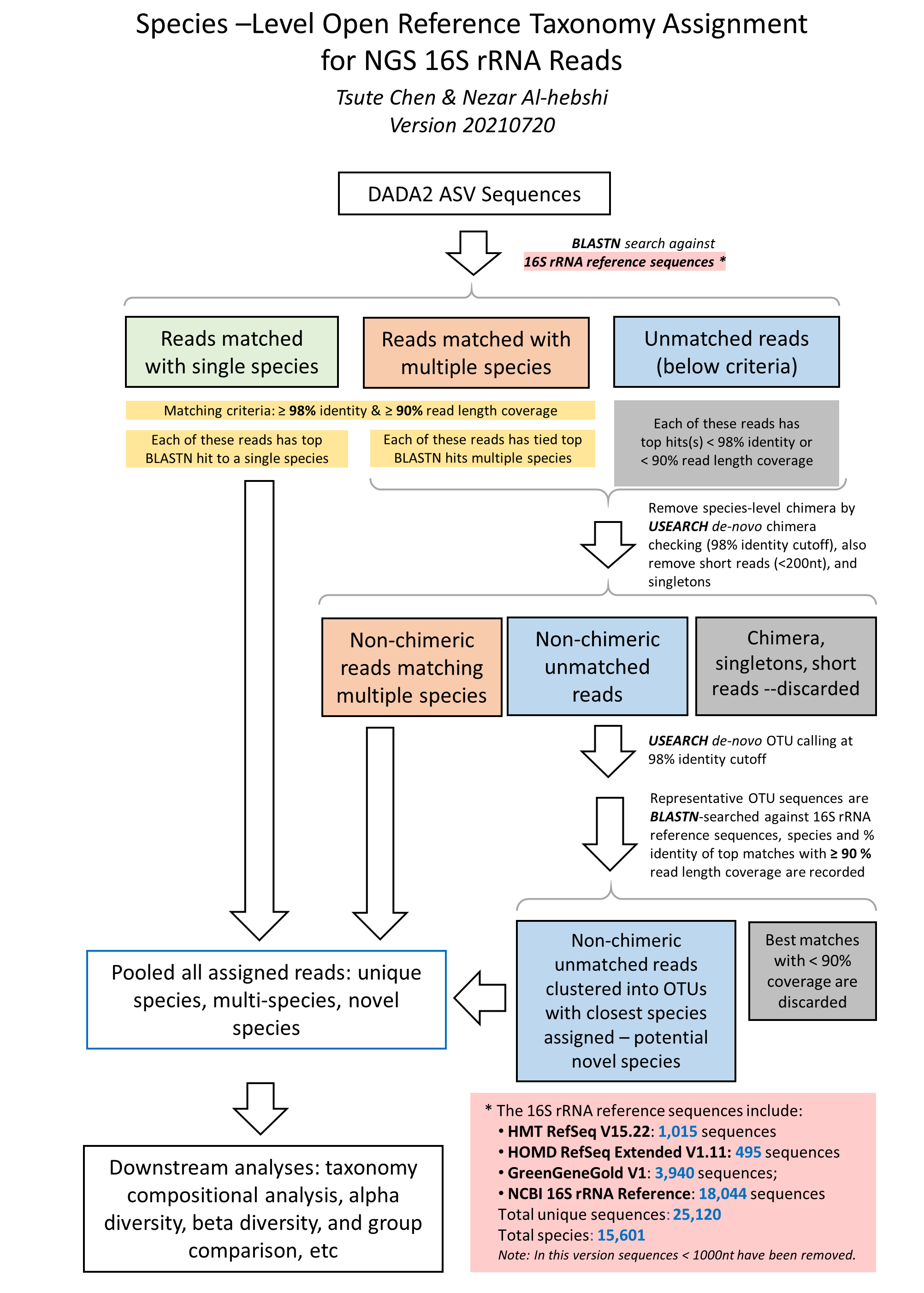
The species-level, open-reference 16S rRNA NGS reads taxonomy assignment pipeline

Version 20210310
 

1. Raw sequences reads in FASTA format were BLASTN-searched against a combined set of 16S rRNA reference sequences. It consists of MOMD (version 0.1), the HOMD (version 15.2 http://www.homd.org/index.php?name=seqDownload&file&type=R ), HOMD 16S rRNA RefSeq Extended Version 1.1 (EXT), GreenGene Gold (GG) (http://greengenes.lbl.gov/Download/Sequence_Data/Fasta_data_files/gold_strains_gg16S_aligned.fasta.gz) , and the NCBI 16S rRNA reference sequence set (https://ftp.ncbi.nlm.nih.gov/blast/db/16S_ribosomal_RNA.tar.gz). These sequences were screened and combined to remove short sequences (<1000nt), chimera, duplicated and sub-sequences, as well as sequences with poor taxonomy annotation (e.g., without species information). This process resulted in 1,015 from HOMD V15.22, 495 from EXT, 3,940 from GG and 18,044 from NCBI, a total of 25,120 sequences. Altogether these sequence represent a total of 15,601 oral and non-oral microbial species.

The NCBI BLASTN version 2.7.1+ (Zhang et al, 2000) was used with the default parameters. Reads with ≥ 98% sequence identity to the matched reference and ≥ 90% alignment length (i.e., ≥ 90% of the read length that was aligned to the reference and was used to calculate the sequence percent identity) were classified based on the taxonomy of the reference sequence with highest sequence identity. If a read matched with reference sequences representing more than one species with equal percent identity and alignment length, it was subject to chimera checking with USEARCH program version v8.1.1861 (Edgar 2010). Non-chimeric reads with multi-species best hits were considered valid and were assigned with a unique species notation (e.g., spp) denoting unresolvable multiple species.

2. Unassigned reads (i.e., reads with < 98% identity or < 90% alignment length) were pooled together and reads < 200 bases were removed. The remaining reads were subject to the de novo operational taxonomy unit (OTU) calling and chimera checking using the USEARCH program version v8.1.1861 (Edgar 2010). The de novo OTU calling and chimera checking was done using 98% as the sequence identity cutoff, i.e., the species-level OTU. The output of this step produced species-level de novo clustered OTUs with 98% identity. Representative reads from each of the OTUs/species were then BLASTN-searched against the same reference sequence set again to determine the closest species for these potential novel species. These potential novel species were pooled together with the reads that were signed to specie-level in the previous step, for down-stream analyses.

Reference:
Edgar RC. Search and clustering orders of magnitude faster than BLAST. Bioinformatics. 2010 Oct 1;26(19):2460-1. doi: 10.1093/bioinformatics/btq461. Epub 2010 Aug 12. PubMed PMID: 20709691.

3. Designations used in the taxonomy:

	1) Taxonomy levels are indicated by these prefixes:
	
	   k__: domain/kingdom
	   p__: phylum
	   c__: class
	   o__: order
	   f__: family
	   g__: genus  
	   s__: species
	
	   Example: 
	
	   k__Bacteria;p__Firmicutes;c__Clostridia;o__Clostridiales;f__Lachnospiraceae;g__Blautia;s__faecis
		
	2) Unique level identified – known species:
	   
	   k__Bacteria;p__Firmicutes;c__Clostridia;o__Clostridiales;f__Lachnospiraceae;g__Roseburia;s__hominis
	
	   The above example shows some reads match to a single species (all levels are unique)
	
	3) Non-unique level identified – known species:

	   k__Bacteria;p__Firmicutes;c__Clostridia;o__Clostridiales;f__Lachnospiraceae;g__Roseburia;s__multispecies_spp123_3
	   
	   The above example “s__multispecies_spp123_3” indicates certain reads equally match to 3 species of the 
	   genus Roseburia; the “spp123” is a temporally assigned species ID.
	
	   k__Bacteria;p__Firmicutes;c__Clostridia;o__Clostridiales;f__Lachnospiraceae;g__multigenus;s__multispecies_spp234_5
	   
	   The above example indicates certain reads match equally to 5 different species, which belong to multiple genera.; 
	   the “spp234” is a temporally assigned species ID.
	
	4) Unique level identified – unknown species, potential novel species:
	   
	   k__Bacteria;p__Firmicutes;c__Clostridia;o__Clostridiales;f__Lachnospiraceae;g__Roseburia;s__ hominis_nov_97%
	   
	   The above example indicates that some reads have no match to any of the reference sequences with 
	   sequence identity ≥ 98% and percent coverage (alignment length)  ≥ 98% as well. However this groups 
	   of reads (actually the representative read from a de novo  OTU) has 96% percent identity to 
	   Roseburia hominis, thus this is a potential novel species, closest to Roseburia hominis. 
	   (But they are not the same species).
	
	5) Multiple level identified – unknown species, potential novel species:
	   k__Bacteria;p__Firmicutes;c__Clostridia;o__Clostridiales;f__Lachnospiraceae;g__Roseburia;s__ multispecies_sppn123_3_nov_96%
	
	   The above example indicates that some reads have no match to any of the reference sequences 
	   with sequence identity ≥ 98% and percent coverage (alignment length)  ≥ 98% as well. 
	   However this groups of reads (actually the representative read from a de novo  OTU) 
	   has 96% percent identity equally to 3 species in Roseburia. Thus this is no single 
	   closest species, instead this group of reads match equally to multiple species at 96%. 
	   Since they have passed chimera check so they represent a novel species. “sppn123” is a 
	   temporary ID for this potential novel species. 

 
4. The taxonomy assignment algorithm is illustrated in this flow char below:


Read Taxonomy Assignment - Result Summary *

CodeCategoryMPC=0% (>=1 read)MPC=0.01%(>=969 reads)
ATotal reads10,017,20710,017,207
BTotal assigned reads9,690,3799,690,379
CAssigned reads in species with read count < MPC056,530
DAssigned reads in samples with read count < 50000
ETotal samples7474
FSamples with reads >= 5007474
GSamples with reads < 50000
HTotal assigned reads used for analysis (B-C-D)9,690,3799,633,849
IReads assigned to single species8,923,8688,894,855
JReads assigned to multiple species163,302157,427
KReads assigned to novel species603,209581,567
LTotal number of species1,28356
MNumber of single species56532
NNumber of multi-species6611
ONumber of novel species65213
PTotal unassigned reads326,828326,828
QChimeric reads1,0681,068
RReads without BLASTN hits111111
SOthers: short, low quality, singletons, etc.325,649325,649
A=B+P=C+D+H+Q+R+S
E=F+G
B=C+D+H
H=I+J+K
L=M+N+O
P=Q+R+S
* MPC = Minimal percent (of all assigned reads) read count per species, species with read count < MPC were removed.
* Samples with reads < 500 were removed from downstream analyses.
* The assignment result from MPC=0.1% was used in the downstream analyses.


Read Taxonomy Assignment - ASV Species-Level Read Counts Table

This table shows the read counts for each sample (columns) and each species identified based on the ASV sequences. The downstream analyses were based on this table.
SPIDTaxonomyN1N2N3N4N5N6N7N8N9O13O14O15O16O17O18O19O20O21O22O23O24O25O26O27O28O29O30O31O32O33O34O35O36O37O38O39O40O41O42O43O44O57O58O59O60O61O62O63O64O65O66O67O68O69O70O71O72O73O74O75O76O77O78O79O80O81O82O83O84O85O86O87O88P1
SP1Bacteria;Firmicutes;Bacilli;Lactobacillales;Streptococcaceae;Streptococcus;danieliae591444495508456528636104919382120091312096402479738127537476656533210271410515792430122973154899144909288686662975971189009999031208821725349908516543219177269026135749957051508275287081227112823447001877142268292433692528902150661615022052920919325288515368510983212206313608411681615947415646810052716971126852250738771910729974669105222588091267471273959796472413146336121688109960302351592
SP10Bacteria;Firmicutes;Bacilli;Bacillales;Staphylococcaceae;Mammaliicoccus;sciuri754218479978258264751109835520449748863617124861460281845018812201432110221247946773142890913127057343714516185140179052111741174377371320185429437431853344235
SP111Bacteria;Firmicutes;Clostridia;Eubacteriales;Clostridiaceae;Clostridium;disporicum125563347271791018611522165162833172410158961031231114913441529187554791023238117022715332321508162110182461520127311334
SP12Bacteria;Proteobacteria;Gammaproteobacteria;Enterobacterales;Enterobacteriaceae;Shigella;boydii353211844714328254450409768400962215570131210630220175454811432510114016910440169304570199009110541243383169
SP13Bacteria;Actinobacteria;Actinomycetia;Actinomycetales;Propionibacteriaceae;Cutibacterium;acnes113583201514660518774239214054448559112640657419703543557923210118672713541001095553910989902229843484144258154128263649461901611387861010884326752107907313259292384449029217105
SP16Bacteria;Proteobacteria;Gammaproteobacteria;Enterobacterales;Enterobacteriaceae;Escherichia;coli113984909212649331731860815691291932150631622221136231924171310812116407775292835191497355927812124111261810102612019123706927823171510801201185142130190
SP17Bacteria;Proteobacteria;Gammaproteobacteria;Enterobacterales;Enterobacteriaceae;Shigella;sonnei3239147176643042651353848830101241116236304810859297411919251074113334011511226111194155700367032322107610444103541258
SP18Bacteria;Firmicutes;Tissierellia;Tissierellales;Peptoniphilaceae;Finegoldia;magna00001000111000011000002300010003000160028100576224425350000500000113000000060000
SP2Bacteria;Firmicutes;Bacilli;Lactobacillales;Enterococcaceae;Enterococcus;faecalis001986130130855059511110813041242293511813257901317102615500230150004225030263222010012001801362389
SP22Bacteria;Proteobacteria;Alphaproteobacteria;Hyphomicrobiales;Phyllobacteriaceae;Phyllobacterium;myrsinacearum1851317052291268541288823782556477828175124026275830106135234046152318256104241118836416269143103784411131640024211912233538014160317
SP28Bacteria;Verrucomicrobia;Verrucomicrobiae;Verrucomicrobiales;Akkermansiaceae;Akkermansia;muciniphila10811892961329819324214921358515899187249309176145481221373711193133817415798223192725614418439102652210223292534
SP29Bacteria;Firmicutes;Bacilli;Bacillales;Staphylococcaceae;Staphylococcus;ureilyticus0034030014221009128885130217922021669906931790212296121214415247300861510063205100420104121718891231540735247154832
SP3Bacteria;Firmicutes;Bacilli;Lactobacillales;Lactobacillaceae;Limosilactobacillus;fermentum1029221003763141691210001002027211016301111031411110801000003000002050041011404100435611
SP30Bacteria;Proteobacteria;Gammaproteobacteria;Enterobacterales;Enterobacteriaceae;Shigella;flexneri101491038815673154910592210110001000001924100000160000000100110000000100220733100025243820
SP33Bacteria;Proteobacteria;Gammaproteobacteria;Enterobacterales;Enterobacteriaceae;Citrobacter;koseri011917310916611116363132100030000092011000090000000100010000000000010047010100200315
SP4Bacteria;Firmicutes;Bacilli;Lactobacillales;Streptococcaceae;Streptococcus;sp._MOT-0126674120141326323194431133364911271403633494851913524671182114456311033123621725018521537123531856522321249118881948521684853983628521531485659637412739511224559373583420175392591271260297209888501146093572021037026031571421151271120196744538283345798974
SP40Bacteria;Proteobacteria;Gammaproteobacteria;Enterobacterales;Enterobacteriaceae;Escherichia;fergusonii3828322492241298693114004009964143007240051191230610049012251010055001110157001010550231056610061239
SP41Bacteria;Firmicutes;Bacilli;Lactobacillales;Streptococcaceae;Streptococcus;mitis1063905331753200320120651010611154960100007100030271000100710020002000601110010230631
SP42Bacteria;Proteobacteria;Alphaproteobacteria;Rhizobiales;Rhizobiaceae;Mesorhizobium;huakuii7411391748830126584020003428200011000000000000002001200020100000100100000001200010001
SP49Bacteria;Firmicutes;Bacilli;Bacillales;Listeriaceae;Listeria;monocytogenes2635272114475881940401032217137013011003304050601110503000105000000091400132063191256370
SP5Bacteria;Firmicutes;Bacilli;Lactobacillales;Lactobacillaceae;Ligilactobacillus;murinus5022627191854204638320968345881847725402479842362274590033086672094640083971414726014203083151165908586208471155213942119368236481489341502001215412626870618910347544932327358734116713998292539198561534125367286567844
SP51Bacteria;Actinobacteria;Actinomycetia;Corynebacteriales;Corynebacteriaceae;Corynebacterium;pilbarense2112477506087278000004030024030200001310110120008163024230101000000662100010010000
SP54Bacteria;Firmicutes;Clostridia;Clostridiales;Peptoniphilaceae;Peptoniphilus;lacydonensis00001000360000400000003000000070000700460001079124900121260000400000229000001020000
SP58Bacteria;Actinobacteria;Actinomycetia;Actinomycetales;Propionibacteriaceae;Cutibacterium;granulosum0013231288266138863125802001232111000202032000440015872216864210108100211544100000040000
SP60Bacteria;Firmicutes;Bacilli;Bacillales;Staphylococcaceae;Staphylococcus;hominis2111618309262583930211725105003100001100032111100422121330020000100057412821001320101
SP63Bacteria;Actinobacteria;Actinomycetia;Corynebacteriales;Corynebacteriaceae;Corynebacterium;tuberculostearicum7550531475212421692000201111006151400200233010510022010960781231330003000003493001100130000
SP68Bacteria;Proteobacteria;Gammaproteobacteria;Enterobacterales;Enterobacteriaceae;Enterobacter;sp._MOT-050002301140153358136612900212000000200201033800100004002000020010030026105728201022211210
SP69Bacteria;Firmicutes;Bacilli;Lactobacillales;Streptococcaceae;Streptococcus;chosunense8310166400819773983000040100200573001000162010010200000007002000062000400500160007202
SP76Bacteria;Actinobacteria;Actinomycetia;Corynebacteriales;Corynebacteriaceae;Corynebacterium;mucifaciens24326206646933199200002031004200010000000030000001002010200000010022311010000101000
SP77Bacteria;Deinococcus-Thermus;Deinococci;Thermales;Thermaceae;Thermus;thermophilus19413020778506010000100200021000100000010044101000302031000020000003200000031000
SP78Bacteria;Firmicutes;Bacilli;Bacillales;Staphylococcaceae;Mammaliicoccus;lentus10300002007260231112213944124441395441514232640219572412119172040032002012170051040012031783091140411470
SP93Bacteria;Proteobacteria;Gammaproteobacteria;Enterobacterales;Enterobacteriaceae;Salmonella;enterica1231880118010037005106000001020406412430120102210401000002000001001102120211110015866
SPN108Bacteria;Firmicutes;Bacilli;Lactobacillales;Streptococcaceae;Streptococcus;danieliae_nov_97.379%0101420141500113825385807243141782178214131277741291286250521127452379568825131164173535373106905877281494567054384549135841193149717629422831497810771188865128118131328475356108446113801285113551142965817527115427538765913019648337198653125291033813905228656
SPN13Bacteria;Firmicutes;Bacilli;Lactobacillales;Streptococcaceae;Streptococcus;danieliae_nov_96.787%1101011704163121726051386936472959655091742477925891599952173100251122902211356292390103038527321903222114941558374240313379114739198631023684200955526148349726491663660927953524432929559830783162567930411458435543846145891762
SPN131Bacteria;Firmicutes;Bacilli;Lactobacillales;Streptococcaceae;Streptococcus;danieliae_nov_93.952%110002505640468917710679711526331113582788256250310308252638075419493954737069779975280115846533383044973143920308060016027011201201604439348553251517894026618510243871700
SPN162Bacteria;Bacteroidetes;Bacteroidia;Bacteroidales;Muribaculaceae;Muribaculaceae_[G-1];bacterium_MOT-129_nov_91.870%8211121251115813298675618971210913613111214561101356248282898165136758531186311110041033858561344653366
SPN216Bacteria;Actinobacteria;Actinomycetia;Actinomycetales;Propionibacteriaceae;Cutibacterium;granulosum_nov_96.788%00000000000000000000000000000100000000010000213904020000100000000000000000002
SPN248Bacteria;Firmicutes;Bacilli;Lactobacillales;Streptococcaceae;Streptococcus;danieliae_nov_95.582%314150216414152663191374146164203244013225622408235675946141717401416156912671005108684521476366951351941863139254161512171071155318741562967148816092223295187010771188839230685911721978973442152815581510217628321
SPN269Bacteria;Firmicutes;Tissierellia;Tissierellales;Peptoniphilaceae;Anaerococcus;octavius_nov_94.583%00001000150000000010000000000010000100014000020210581010000100000000000000010000
SPN363Bacteria;Firmicutes;Bacilli;Lactobacillales;Streptococcaceae;Streptococcus;danieliae_nov_93.387%0300000001153343394410530152637629024014113810283372242101081361241484757268167142210193241495923192100501182411548125310720915100614316291541132412748426317211
SPN43Bacteria;Bacteroidetes;Chitinophagia;Chitinophagales;Chitinophagaceae;Segetibacter;koreensis_nov_89.733%20032116703000000100000002000000010000000100000001000000020000000000000002000
SPN482Bacteria;Bacteroidetes;Bacteroidia;Bacteroidales;Prevotellaceae;Prevotella;shahii_nov_87.903%108735101641382313191118371112371292015446171214121324422121273548226652016161681122241218108301517101820163671018211216813412142139
SPN559Bacteria;Actinobacteria;Actinomycetia;Actinomycetales;Propionibacteriaceae;Cutibacterium;acnes_nov_96.815%00000111000000300000000000000100000000000000217743000000100000001000000010000
SPN571Bacteria;Bacteroidetes;Bacteroidia;Bacteroidales;Muribaculaceae;Duncaniella;freteri_nov_91.751%1143475437810116171682391714199685101714469126121213663242614513318611611319111676739216161526449106301476131215108124
SPN582Bacteria;Bacteroidetes;Bacteroidia;Bacteroidales;Muribaculaceae;Duncaniella;freteri_nov_88.577%14322421153203161868261071356710034101016490577722113125151474523285937441749964945339140534371
SPP12Bacteria;Proteobacteria;Alphaproteobacteria;Rhizobiales;Bradyrhizobiaceae;Bosea;multispecies_spp12_21026211967672410911000000300210000040000010000002010203610000030020000001100000012100
SPP15Bacteria;Firmicutes;Bacilli;Bacillales;Staphylococcaceae;Staphylococcus;multispecies_spp15_25084402134129328187472133062000410020001003000900013000034821010001200202300220000011201
SPP19Bacteria;Proteobacteria;Gammaproteobacteria;Enterobacterales;Enterobacteriaceae;multigenus;multispecies_spp19_215158692619133927882311524006495215611112133015115212240351100104022200200341004112050021402417313272662
SPP24Bacteria;Proteobacteria;Betaproteobacteria;Burkholderiales;Burkholderiaceae;multigenus;multispecies_spp24_852758768315021134300000404100000010001200000000000000020001000100110000000000020003
SPP33Bacteria;Proteobacteria;Betaproteobacteria;Burkholderiales;Burkholderiaceae;Burkholderia;multispecies_spp33_563155911071199263474101001701400000010000301000000001000000020001101100002000100010010
SPP44Bacteria;Firmicutes;Bacilli;Bacillales;Bacillaceae;Bacillus;multispecies_spp44_25766354535708808402020056040141050120000020706301517220013100010021720410310122001083750
SPP49Bacteria;Firmicutes;Bacilli;Bacillales;Staphylococcaceae;Staphylococcus;multispecies_spp49_310401977623791558300000800030400010220001025230000070200100500001004600001100240124254
SPP52Bacteria;Firmicutes;Bacilli;Lactobacillales;Streptococcaceae;Streptococcus;multispecies_spp52_32315383117149910556153100017200001030010100600100004110000050000000210208020200151017001
SPP57Bacteria;Firmicutes;Bacilli;Bacillales;Staphylococcaceae;Staphylococcus;multispecies_spp57_20000010115635940638191615772104129605801411030369212471413319284826260379341231201151012135319041413046270214145316901291227134453
SPP62Bacteria;Proteobacteria;Alphaproteobacteria;Rhizobiales;Rhizobiaceae;multigenus;multispecies_spp62_212134113115143103810000090430000300000006000000130000002130000000610000007000000010000
SPP64Bacteria;Proteobacteria;Betaproteobacteria;Burkholderiales;Burkholderiaceae;Burkholderia;multispecies_spp64_317013063929885424711397361302931078290413618595131216660214915133000673011113101156091643014772181619011601101532013572131433015624121540
 
 
Download OTU Tables at Different Taxonomy Levels
PhylumCount*: Relative**: CLR***:
ClassCount*: Relative**: CLR***:
OrderCount*: Relative**: CLR***:
FamilyCount*: Relative**: CLR***:
GenusCount*: Relative**: CLR***:
SpeciesCount*: Relative**: CLR***:
* Read count
** Relative abundance (count/total sample count)
*** Centered log ratio transformed abundance
;
 
The species listed in the table has full taxonomy and a dynamically assigned species ID specific to this report. When some reads match with the reference sequences of more than one species equally (i.e., same percent identiy and alignmnet coverage), they can't be assigned to a particular species. Instead, they are assigned to multiple species with the species notaton "s__multispecies_spp2_2". In this notation, spp2 is the dynamic ID assigned to these reads that hit multiple sequences and the "_2" at the end of the notation means there are two species in the spp2.

You can look up which species are included in the multi-species assignment, in this table below:


Another type of notation is "s__multispecies_sppn2_2", in which the "n" in the sppn2 means it's a potential novel species because all the reads in this species have < 98% idenity to any of the reference sequences. They were grouped together based on de novo OTU clustering at 98% identity cutoff. And then a representative sequence was chosed to BLASTN search against the reference database to find the closest match (but will still be < 98%). This representative sequence also matched equally to more than one species, hence the "spp" was given in the label.


Taxonomy Bar Plots for All Samples


Taxonomy Bar Plots for Individual Comparison Groups


Comparison No.Comparison NameFamiliesGeneraSpecies
Comparison 1F vs M vs NegativePDFSVGPDFSVGPDFSVG
Comparison 2CMC vs S_mitis vs NegativePDFSVGPDFSVGPDFSVG
Comparison 3Taconic vs Jackson vs NegativePDFSVGPDFSVGPDFSVG


VIII. Analysis - Alpha Diversity


In ecology, alpha diversity (α-diversity) is the mean species diversity in sites or habitats at a local scale. The term was introduced by R. H. Whittaker[1][2] together with the terms beta diversity (β-diversity) and gamma diversity (γ-diversity). Whittaker's idea was that the total species diversity in a landscape (gamma diversity) is determined by two different things, the mean species diversity in sites or habitats at a more local scale (alpha diversity) and the differentiation among those habitats (beta diversity).


References:
Whittaker, R. H. (1960) Vegetation of the Siskiyou Mountains, Oregon and California. Ecological Monographs, 30, 279–338. doi:10.2307/1943563
Whittaker, R. H. (1972). Evolution and Measurement of Species Diversity. Taxon, 21, 213-251. doi:10.2307/1218190


Alpha Diversity Analysis by Rarefaction

Diversity measures are affected by the sampling depth. Rarefaction is a technique to assess species richness from the results of sampling. Rarefaction allows the calculation of species richness for a given number of individual samples, based on the construction of so-called rarefaction curves. This curve is a plot of the number of species as a function of the number of samples. Rarefaction curves generally grow rapidly at first, as the most common species are found, but the curves plateau as only the rarest species remain to be sampled.


References:
Willis AD. Rarefaction, Alpha Diversity, and Statistics. Front Microbiol. 2019 Oct 23;10:2407. doi: 10.3389/fmicb.2019.02407. PMID: 31708888; PMCID: PMC6819366.


Boxplot of Alpha-diversity Indices

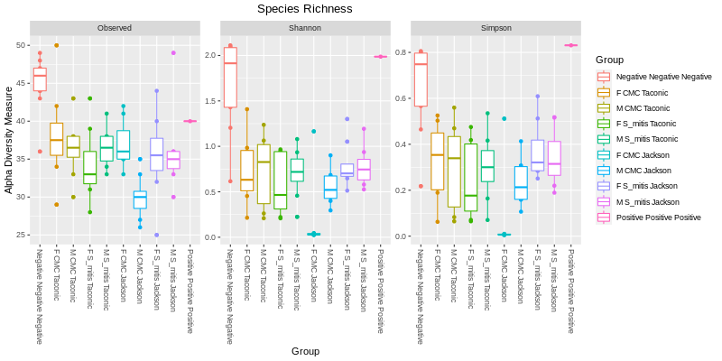
The two main factors taken into account when measuring diversity are richness and evenness. Richness is a measure of the number of different kinds of organisms present in a particular area. Evenness compares the similarity of the population size of each of the species present. There are many different ways to measure the richness and evenness. These measurements are called "estimators" or "indices". Below is a diversity of 3 commonly used indices showing the values for all the samples (dots) and in groups (boxes).

 
Alpha Diversity Box Plots for All Groups


Alpha Diversity Box Plots for Individual Comparisons
 
Comparison 1F vs M vs NegativeView in PDFView in SVG
Comparison 2CMC vs S_mitis vs NegativeView in PDFView in SVG
Comparison 3Taconic vs Jackson vs NegativeView in PDFView in SVG


Group Significance of Alpha-diversity Indices

To test whether the alpha diversity among different comparison groups are different statisticall, we use the Kruskal Wallis H test provided the "alpha-group-significance" fucntion in the QIIME 2 diversity package. Kruskal Wallis H test is the non parametric alternative to the One Way ANOVA. Non parametric means that the test doesn’t assume your data comes from a particular distribution. The H test is used when the assumptions for ANOVA aren’t met (like the assumption of normality). It is sometimes called the one-way ANOVA on ranks, as the ranks of the data values are used in the test rather than the actual data points. The test determines whether the medians of two or more groups are different.

Below are the Kruskal Wallis H test results for each comparison based on three different alpha diversity measures: 1) Observed species (features), 2) Shannon index, and 3) Simpson index.


Comparison 1.F vs M vs NegativeObserved FeaturesShannon IndexSimpson Index
Comparison 2.CMC vs S_mitis vs NegativeObserved FeaturesShannon IndexSimpson Index
Comparison 3.Taconic vs Jackson vs NegativeObserved FeaturesShannon IndexSimpson Index


IX. Analysis - Beta Diversity


NMDS and PCoA Plots

Beta diversity compares the similarity (or dissimilarity) of microbial profiles between different groups of samples. There are many different similarity/dissimilarity metrics. In general, they can be quantitative (using sequence abundance, e.g., Bray-Curtis or weighted UniFrac) or binary (considering only presence-absence of sequences, e.g., binary Jaccard or unweighted UniFrac). They can be even based on phylogeny (e.g., UniFrac metrics) or not (non-UniFrac metrics, such as Bray-Curtis, etc.).

For microbiome studies, species profiles of samples can be compared with the Bray-Curtis dissimilarity, which is based on the count data type. The pair-wise Bray-Curtis dissimilarity matrix of all samples can then be subject to either multi-dimensional scaling (MDS, also known as PCoA) or non-metric MDS (NMDS).

MDS/PCoA is a scaling or ordination method that starts with a matrix of similarities or dissimilarities between a set of samples and aims to produce a low-dimensional graphical plot of the data in such a way that distances between points in the plot are close to original dissimilarities.

NMDS is similar to MDS, however it does not use the dissimilarities data, instead it converts them into the ranks and use these ranks in the calculation.

In our beta diversity analysis, Bray-Curtis dissimilarity matrix was first calculated and then plotted by the PCoA and NMDS separately. Below are beta diveristy results for all groups together:


NMDS and PCoA Plots for All Groups


The above PCoA and NMDS plots are based on count data. The count data can also be transformed into centered log ratio (CLR) for each species. The CLR data is no longer count data and cannot be used in Bray-Curtis dissimilarity calculation. Instead CLR can be compared with Euclidean distances. When CLR data are compared by Euclidean distance, the distance is also called Aitchison distance.

Below are the NMDS and PCoA plots of the Aitchison distances of the samples:


NMDS and PCoA Plots for Individual Comparisons
 
 
Comparison No.Comparison NameNMDAPCoA
Bray-CurtisCLR EuclideanBray-CurtisCLR Euclidean
Comparison 1F vs M vs NegativePDFSVGPDFSVGPDFSVGPDFSVG
Comparison 2CMC vs S_mitis vs NegativePDFSVGPDFSVGPDFSVGPDFSVG
Comparison 3Taconic vs Jackson vs NegativePDFSVGPDFSVGPDFSVGPDFSVG


Interactive 3D PCoA Plots - Bray-Curtis Dissimilarity


Interactive 3D PCoA Plots - Euclidean Distance


Interactive 3D PCoA Plots - Correlation Coefficients


Group Significance of Beta-diversity Indices

To test whether the between-group dissimilarities are significantly greater than the within-group dissimilarities, the "beta-group-significance" function provided in the QIIME 2 "diversity" package was used with PERMANOVA (permutational multivariate analysis of variance) chosen s the group significan testing method.

Three beta diversity matrics were used: 1) Bray–Curtis dissimilarity 2) Correlation coefficient matrix , and 3) Aitchison distance (Euclidean distance between clr-transformed compositions).


Comparison 1.F vs M vs NegativeBray–CurtisCorrelationAitchison
Comparison 2.CMC vs S_mitis vs NegativeBray–CurtisCorrelationAitchison
Comparison 3.Taconic vs Jackson vs NegativeBray–CurtisCorrelationAitchison


X. Analysis - Differential Abundance

16S rRNA next generation sequencing (NGS) generates a fixed number of reads that reflect the proportion of different species in a sample, i.e., the relative abundance of species, instead of the absolute abundance. In Mathematics, measurements involving probabilities, proportions, percentages, and ppm can all be thought of as compositional data. This makes the microbiome read count data “compositional” (Gloor et al, 2017). In general, compositional data represent parts of a whole which only carry relative information (http://www.compositionaldata.com/).

The problem of microbiome data being compositional arises when comparing two groups of samples for identifying “differentially abundant” species. A species with the same absolute abundance between two conditions, its relative abundances in the two conditions (e.g., percent abundance) can become different if the relative abundance of other species change greatly. This problem can lead to incorrect conclusion in terms of differential abundance for microbial species in the samples.

When studying differential abundance (DA), the current better approach is to transform the read count data into log ratio data. The ratios are calculated between read counts of all species in a sample to a “reference” count (e.g., mean read count of the sample). The log ratio data allow the detection of DA species without being affected by percentage bias mentioned above

In this report, a compositional DA analysis tool “ANCOM” (analysis of composition of microbiomes) was used. ANCOM transforms the count data into log-ratios and thus is more suitable for comparing the composition of microbiomes in two or more populations. "ANCOM" generates a table of features with W-statistics and whether the null hypothesis is rejected. The “W” is the W-statistic, or number of features that a single feature is tested to be significantly different against. Hence the higher the "W" the more statistical sifgnificane that a feature/species is differentially abundant.


References:

Gloor GB, Macklaim JM, Pawlowsky-Glahn V, Egozcue JJ. Microbiome Datasets Are Compositional: And This Is Not Optional. Front Microbiol. 2017 Nov 15;8:2224. doi: 10.3389/fmicb.2017.02224. PMID: 29187837; PMCID: PMC5695134.

Mandal S, Van Treuren W, White RA, Eggesbø M, Knight R, Peddada SD. Analysis of composition of microbiomes: a novel method for studying microbial composition. Microb Ecol Health Dis. 2015 May 29;26:27663. doi: 10.3402/mehd.v26.27663. PMID: 26028277; PMCID: PMC4450248.

Lin H, Peddada SD. Analysis of compositions of microbiomes with bias correction. Nat Commun. 2020 Jul 14;11(1):3514. doi: 10.1038/s41467-020-17041-7. PMID: 32665548; PMCID: PMC7360769.


ANCOM Differential Abundance Analysis

 
ANCOM Results for Individual Comparisons
Comparison No.Comparison Name
Comparison 1.F vs M vs Negative
Comparison 2.CMC vs S_mitis vs Negative
Comparison 3.Taconic vs Jackson vs Negative


ANCOM-BC Differential Abundance Analysis


Starting with version V1.2, we also include the results of ANCOM-BC (Analysis of Compositions of Microbiomes with Bias Correction) (Lin and Peddada 2020). ANCOM-BC is an updated version of "ANCOM" that: (a) provides statistically valid test with appropriate p-values, (b) provides confidence intervals for differential abundance of each taxon, (c) controls the False Discovery Rate (FDR), (d) maintains adequate power, and (e) is computationally simple to implement. The bias correction (BC) addresses a challenging problem of the bias introduced by differences in the sampling fractions across samples. This bias has been a major hurdle in performing DA analysis of microbiome data. ANCOM-BC estimates the unknown sampling fractions and corrects the bias induced by their differences among samples. The absolute abundance data are modeled using a linear regression framework.

References:

Lin H, Peddada SD. Analysis of compositions of microbiomes with bias correction. Nat Commun. 2020 Jul 14;11(1):3514. doi: 10.1038/s41467-020-17041-7. PMID: 32665548; PMCID: PMC7360769.


ANCOM-BC Results for Individual Comparisons
 
Comparison No.Comparison Name
Comparison 1.F vs M vs Negative
Comparison 2.CMC vs S_mitis vs Negative
Comparison 3.Taconic vs Jackson vs Negative


LEfSe - Linear Discriminant Analysis Effect Size

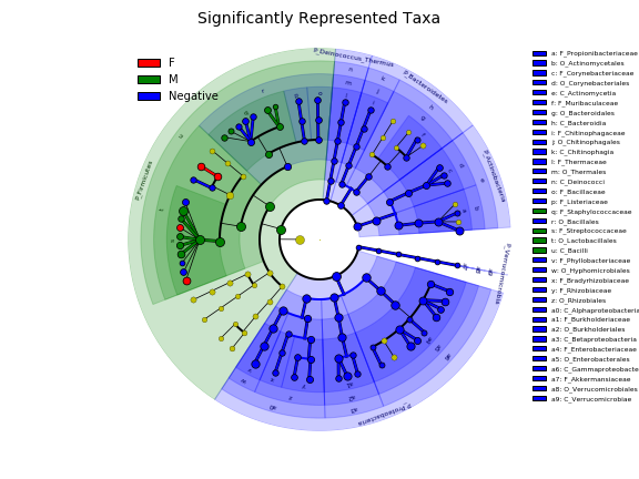
LEfSe (Linear Discriminant Analysis Effect Size) is an alternative method to find "organisms, genes, or pathways that consistently explain the differences between two or more microbial communities" (Segata et al., 2011). Specifically, LEfSe uses rank-based Kruskal-Wallis (KW) sum-rank test to detect features with significant differential (relative) abundance with respect to the class of interest. Since it is rank-based, instead of proportional based, the differential species identified among the comparison groups is less biased (than percent abundance based).

Reference:

Segata N, Izard J, Waldron L, Gevers D, Miropolsky L, Garrett WS, Huttenhower C. Metagenomic biomarker discovery and explanation. Genome Biol. 2011 Jun 24;12(6):R60. doi: 10.1186/gb-2011-12-6-r60. PMID: 21702898; PMCID: PMC3218848.

 
F vs M vs Negative


LEfSe Results for All Comparisons
 
Comparison No.Comparison Name
Comparison 1.F vs M vs Negative
Comparison 2.CMC vs S_mitis vs Negative
Comparison 3.Taconic vs Jackson vs Negative


XI. Analysis - Heatmap Profile


Species vs Sample Abundance Heatmap for All Samples


Heatmaps for Individual Comparisons

 
A) Two-way clustering - clustered on both columns (Samples) and rows (organism)
Comparison No.Comparison NameFamily LevelGenus LevelSpecies Level
Comparison 1F vs M vs NegativePDFSVGPDFSVGPDFSVG
Comparison 2CMC vs S_mitis vs NegativePDFSVGPDFSVGPDFSVG
Comparison 3Taconic vs Jackson vs NegativePDFSVGPDFSVGPDFSVG
 
 
B) One-way clustering - clustered on rows (organism) only
Comparison No.Comparison NameFamily LevelGenus LevelSpecies Level
Comparison 1F vs M vs NegativePDFSVGPDFSVGPDFSVG
Comparison 2CMC vs S_mitis vs NegativePDFSVGPDFSVGPDFSVG
Comparison 3Taconic vs Jackson vs NegativePDFSVGPDFSVGPDFSVG
 
 
C) No clustering
Comparison No.Comparison NameFamily LevelGenus LevelSpecies Level
Comparison 1F vs M vs NegativePDFSVGPDFSVGPDFSVG
Comparison 2CMC vs S_mitis vs NegativePDFSVGPDFSVGPDFSVG
Comparison 3Taconic vs Jackson vs NegativePDFSVGPDFSVGPDFSVG


XII. Analysis - Network Association

To analyze the co-occurrence or co-exclusion between microbial species among different samples, network correlation analysis tools are usually used for this purpose. However, microbiome count data are compositional. If count data are normalized to the total number of counts in the sample, the data become not independent and traditional statistical metrics (e.g., correlation) for the detection of specie-species relationships can lead to spurious results. In addition, sequencing-based studies typically measure hundreds of OTUs (species) on few samples; thus, inference of OTU-OTU association networks is severely under-powered. Here we use SPIEC-EASI (SParse InversE Covariance Estimation for Ecological Association Inference), a statistical method for the inference of microbial ecological networks from amplicon sequencing datasets that addresses both of these issues (Kurtz et al., 2015). SPIEC-EASI combines data transformations developed for compositional data analysis with a graphical model inference framework that assumes the underlying ecological association network is sparse. SPIEC-EASI provides two algorithms for network inferencing – 1) Meinshausen-Bühlmann's neighborhood selection (MB method) and inverse covariance selection (GLASSO method, i.e., graphical least absolute shrinkage and selection operator). This is fundamentally distinct from SparCC, which essentially estimate pairwise correlations. In addition to these two methods, we provide the results of a third method - SparCC (Sparse Correlations for Compositional Data)(Friedman & Alm 2012), which is also a method for inferring correlations from compositional data. SparCC estimates the linear Pearson correlations between the log-transformed components.


References:

Kurtz ZD, Müller CL, Miraldi ER, Littman DR, Blaser MJ, Bonneau RA. Sparse and compositionally robust inference of microbial ecological networks. PLoS Comput Biol. 2015 May 7;11(5):e1004226. doi: 10.1371/journal.pcbi.1004226. PMID: 25950956; PMCID: PMC4423992.

Friedman J, Alm EJ. Inferring correlation networks from genomic survey data. PLoS Comput Biol. 2012;8(9):e1002687. doi: 10.1371/journal.pcbi.1002687. Epub 2012 Sep 20. PMID: 23028285; PMCID: PMC3447976.


SPIEC-EASI Network Inference by Neighborhood Selection (MB Method)


Association Network Inference by SparCC


Copyright FOMC 2023