SAMPLE RESULTS |
| 1. |
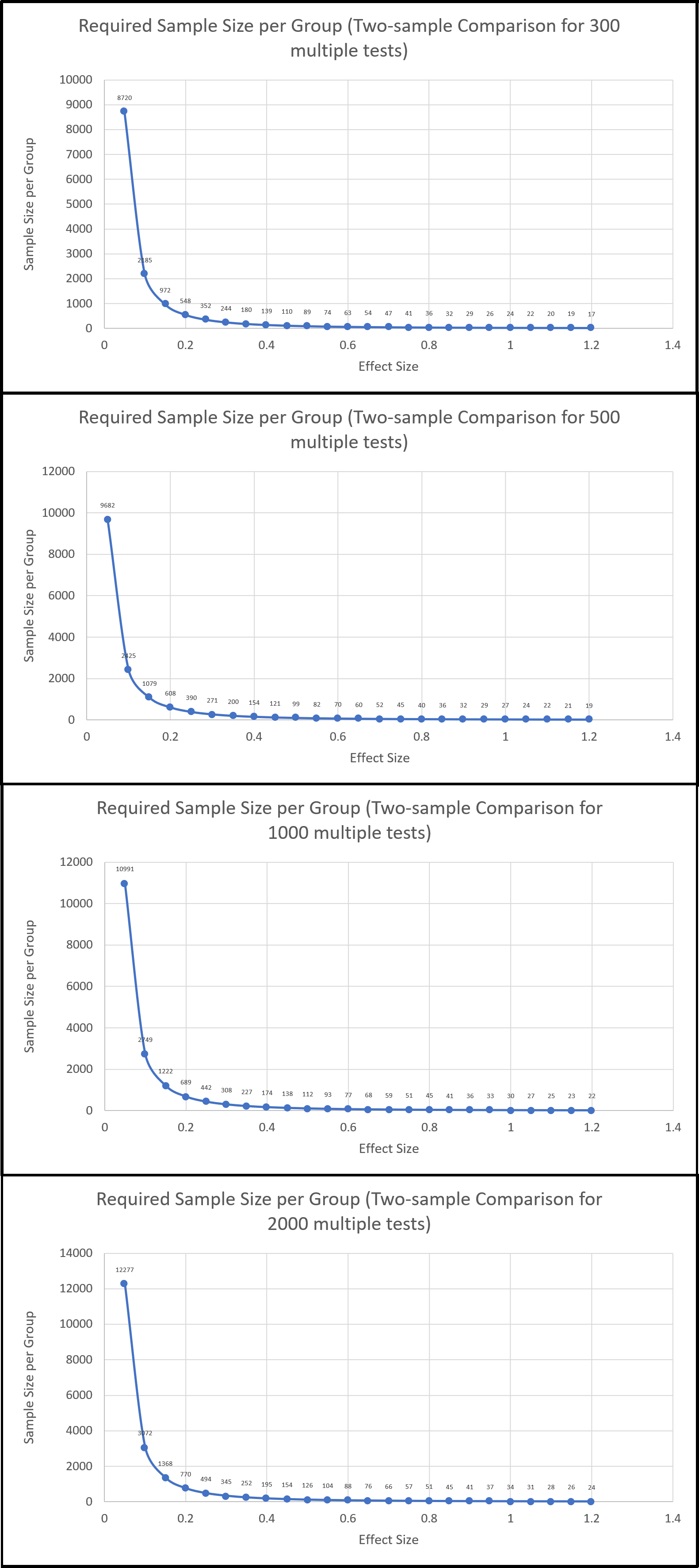
Sample size calculation. In the early stage of a project, experiemtal design is of crutial importance. For microbiomic studies, it is necessary to
consider the desired false discovery rate, number of microbial features detected, and the effect size to determine a adequate sample size in order to
achieve signficant conslusion for hypothesis testings. Below is an example of such calculation. We will assisst you with the experimental design to come up with
a reasonable sample size, ideally within the constraint of the budget.
|
| |
| |  |
| |
| 2. |
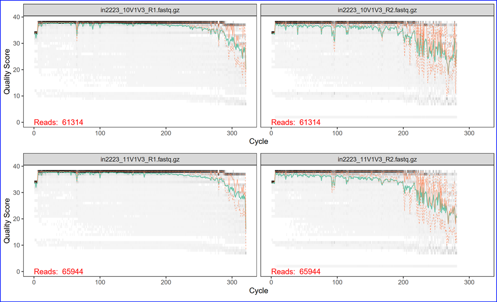
DADA2 Read Quality Plots. The Illumina sequencer sequences both ends of a DNA amplicon
at the same time, expanding the sequence length and span. If the two reads overlap enough, we
can also merge them together into a single sequence from each pair of the reads. We will process
them separately first for quality filtering and later merge them together for downstream
analysis. The graph below is a heat map of the frequency of each quality score at each base
position. The median quality score at each position is shown by the green line, and the
quartiles of the quality score distribution by the orange lines. The red line shows the
scaled proportion of reads that extend to at least that position. The purpose of examining
these quality plots is to help us pick a trimming length for the reads. Usually the sequence
quality degrades more rapidly toward the end of the read, this is especially true for R2.
|
| |
| |  |
| |
| 3. |
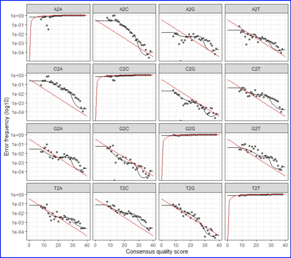
DADA2 Sequence Error Model for ASV inferring. There are a total of 12 possible nucleotide
transition (e.g., A=>C, A=>G, etc). The plot shows the pair-wise transition of A, T, C and G
(including self). The dots indicate the observed error rates for each consensus quality
score. The black lines are the estimated error rates after convergence of the
machine-learning algorithm. The red lines are the error rates expected under the
nominal definition of the Q-score. Ideally, we want to see a good fit between the black
dots and the black line. As you can see the higher the quality scores the lower the error frequencies.
|
| |
| |  |
| |
| 4. |
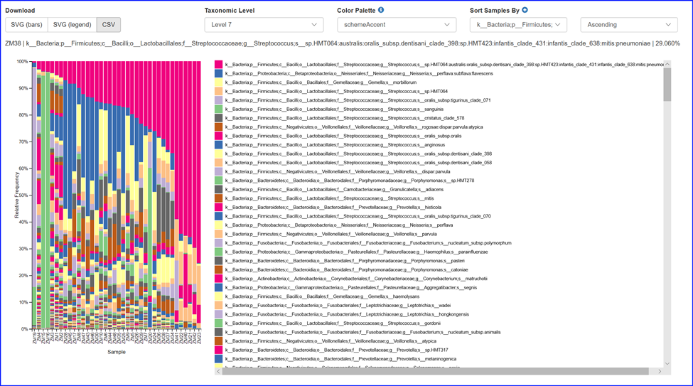
Interactive compositional bar plot from phylum to species. After the taxonomy assignment of the ASVs,
we will offer an interactive compositional bar plot that is capable of showing microbial community composition
bar plots from phylum and species level. The plot can be easily sorted and downloaded and saved for additional modification.
Please click on the example barchart below to try it.
|
| |
| |  |
| |
| 5. |
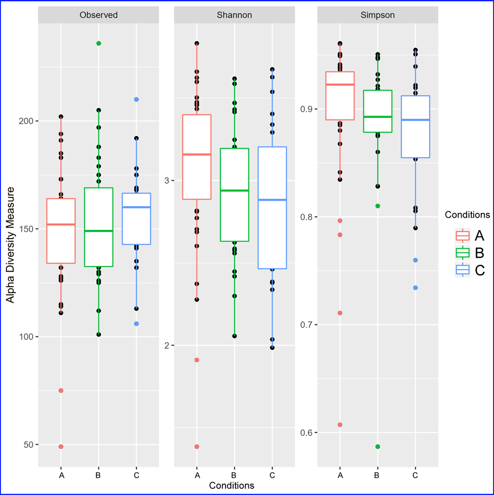
Alpha diversity. Alpha diversity (α-diversity) is the microbial diversity in samples or groups of samples.
Diversity can be measured based on either the number of species (richness) and/or the abundance of species
(evenness - proportions of species). Often researchers use the values given by one or more diversity indices,
such as species richness (which is simply a count of observed species), the Shannon index or the Simpson index
(which also takes into account species proportional abundances).
Below is an example of microbial diversity measured by 3 different diversity indeces - observed, Shannon and Simpson.
|
| |
| |  |
| |
| 6. |
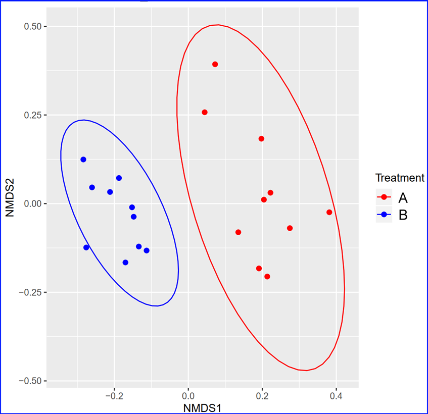
Beta diversity. Beta diversity (β-diversity) is the comparison of microbial diversity between two or
more groups of samples. For beta diversity, we are interested in how the composition of the microbiome
differs from one group of samples to another. There are many measurements to calculate the distance or
similarity between two given groups of samples. One common tool to do this is non-metric multidimensional
scaling, or NMDS. NMDS collapses information from multiple dimensions (e.g, from multiple communities,
sites, etc.) into just a few, so that they can be visualized and interpreted. Unlike other ordination
techniques that rely on (primarily Euclidean) distances, such as Principal Coordinates Analysis, NMDS uses
rank orders, and thus is an extremely flexible technique that can accommodate a variety of different kinds of data.
Below is an example of Non-metric multi-dimensional scaling (NMDS) plot that shows the separation of two groups of samples in the two dimension space.
|
| |
| |  |
| |
| 7. |
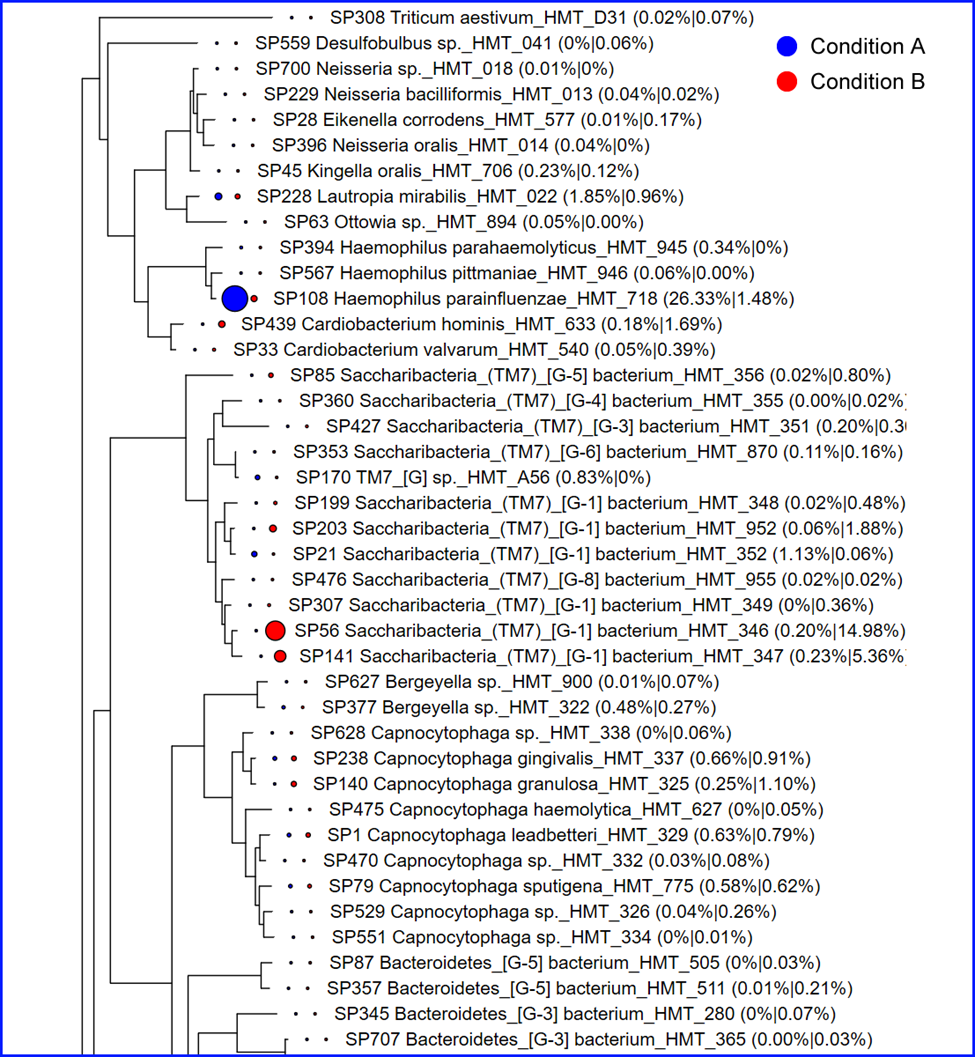
Phylogenetic trees with abundance. We also provide abundance data on a phylogenetic tree dynamically
constructed from the species detected in your data. Often times it is useful to examine the microbes with their
phylogenetic relatedness. In the figure below, the conditions are colored differently and the size of the
circles is proportional to the percent abundance
|
| |
| |  |
| |
| 8. |
QIIME2 results. We also offer many additional results generated by the
QIIME2 pipeline, including:
1) Feature summary
2) Interative alpha rarefaction chart
3) Interative composition bar chart
4) Sample vs. species heatmap
5) PCOA plot
6) Core features
|
| |
| | We can offer more results available through QIIME2 pipeline upon request.
For more detailed information about QIIME2,
please visit the QIIME2 web site. |
| |
| 9. |
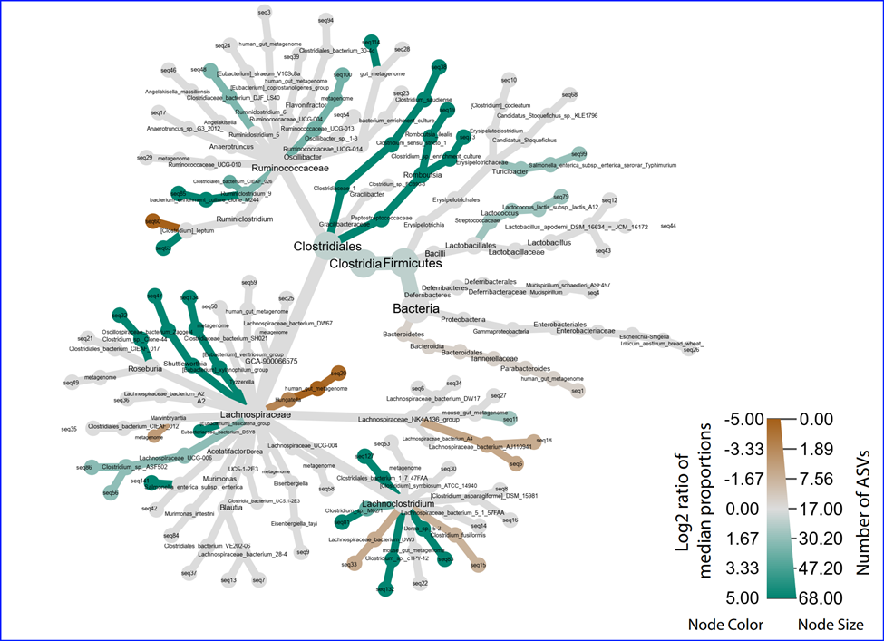
Differential abundance between two conditions - Metacoder display. To study bacterial species that
are differentially abundant in different conditions, we present such information by using
Metacoder -
an R package for easily parsing, manipulating, and graphing publication-ready plots of hierarchical data.
In the sample Metacorder result, different abundance information is shown in a heat tree with the taxonomy
hierarchy and colors used to present higher (green) or lower (brown) abundance when comparing two conditions.
|
| |
| |  |
| |
| 10. |
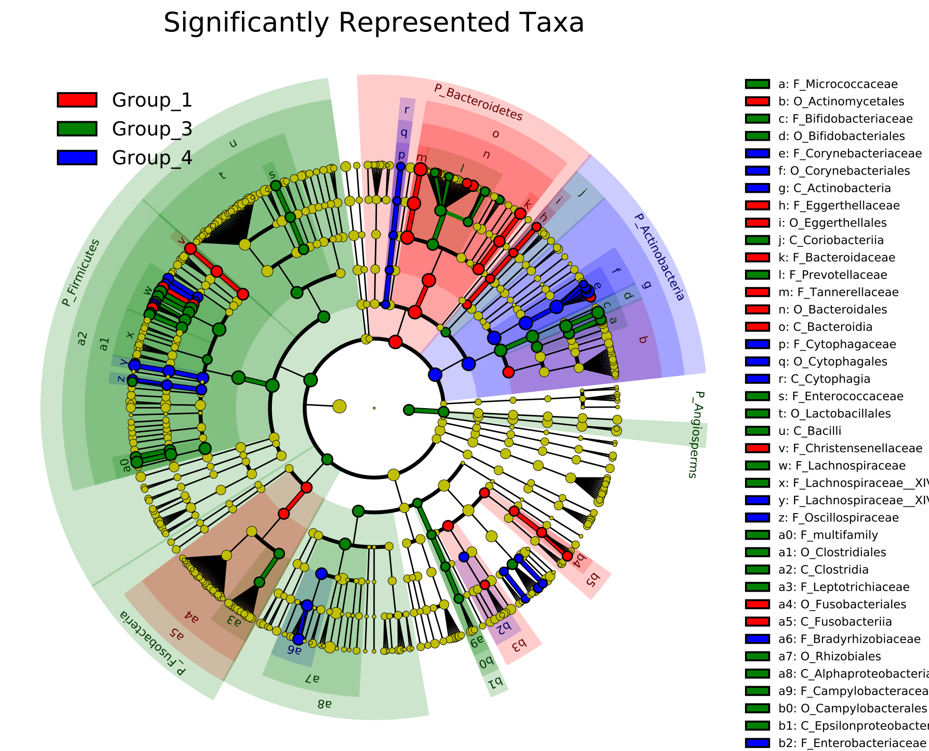
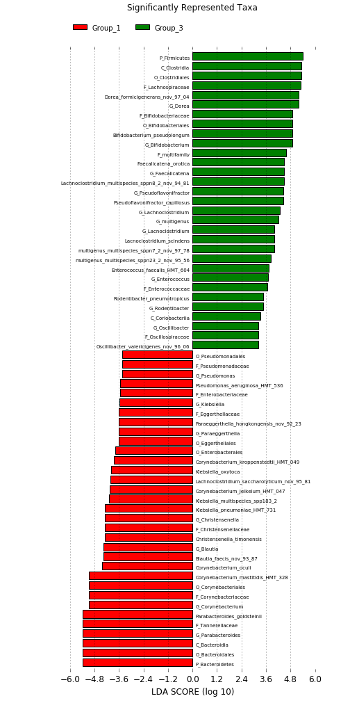
Linear discriminant analysis effect size (LEfSe) analysis to identify differences in abundant taxa.
Differential abundance can also be studied using the LEfSe (Linear discriminant analysis effect size) tool.
LEfSe first identifies features that are statistically different among biological classes. LEfSe then tests
whether the difference is driven by differential species in all samples or just one sample in a group.
An effect size score linear discriminant analysis (LDA) is calculated for each species to represent the
contribution of a particular species that drives the difference.
Below is a sample LEfSe result that identifies differentially abundance genera that contribute to the difference between two microbial communities .
|
| |
| |  |
| |
| |
| |  |
| |